9 Domain Knowledge

Feedback wanted

This book is work in progress. We are happy to receive your feedback via science-book@christophmolnar.com

Machine learning algorithms learn models from data without needing much input from us. At least compared to other modeling approaches. But what about all the domain knowledge that we already have? Having models learn from data is the opposite of using domain knowledge – we let an algorithm identify the relevant patterns and differentiate between signal and noise.

Domain knowledge

Domain knowledge refers to facts that have been established in a field.

Can we use domain knowledge to guide the model? This chapter shows that we can, ranging from the standard steps of translating the problem into a prediction task to more creative means such as designing custom evaluation metrics. The chapter focuses on ways to infuse domain knowledge directly into the model. Less well-known is that we can extract domain knowledge from the model: Domain knowledge constrains the model and affects its performance, which gives us information on how valuable the domain knowledge is for this prediction task. This makes machine learning a two-way street between domain knowledge and predictive performance.

The Ravens struggled to fully integrate machine learning into Raven Science. Even if the tornado warning system was a success, they had to dismiss most of their domain knowledge and let the machine learn from scratch, or so it seemed. How wasteful, thought Krahrah. This was an insult to previous raven scientists and the knowledge they had generated. Even worse, the machines didn’t contribute to the great library of raven knowledge but kept their secrets hidden in the algorithms. If only there was a way to integrate knowledge into supervised ML models and maybe even get some knowledge in return.

9.1 Translate the question into a prediction task

The Ravens were wrong. Machine learning models are typically infused with lots of domain knowledge already, even when it may seem otherwise at first. Most domain knowledge comes from “translating” the scientific question into the prediction task. Predicting tornadoes from radar data and not from the number of people reporting knee aches might seem like common sense. But as soon as you get into the details of designing the prediction task, you typically rely on deeper domain knowledge. Designing the prediction task might not always feel like infusing domain knowledge, especially when the prediction task is long established, like in weather forecasting. But for scientific problems that aren’t typically set up as prediction tasks, the translation process allows for a lot of creativity, which should be guided by domain knowledge.

A big part of the translation is creating features and targets. Whether you predict intelligence from the income of the parents or chocolate consumption (Maurage, Heeren, and Pesenti 2013) makes for very different models. But if you are a typical reader of this book, you already know these things. Time to get to the juicy and often overlooked means to infuse domain knowledge.

9.2 Constrain the model

Machine learning is praised for the flexibility to learn any function, but sometimes you might want the opposite and constrain the model. Model constraints are a direct way to incorporate domain knowledge into the learning process. Some examples of constraints that can be put on the relation between features and the prediction:

Monotonicity: The model’s predictions have to increase or decrease monotonically with increasing values of the feature in question. Example: Ensuring credit risk scores increase monotonically with income.
Linearity: Restrict the model to learn a linear relation between prediction and feature(s). Example: Predicting rent, where the price is linearly dependent on the size.
Sparsity: Restrict the number of features to be used for the prediction. Example: In genomic studies, identifying a small subset of genes responsible for a particular disease.
Smoothness: Restrict the predictions to smoothly change when the input changes. Example: Predicting temperature as a function of altitude, where abrupt changes are not expected.
Cyclicity: A smoothness constraint that ensures that the predictions for the low and high end of a feature “meet”. Example: Predicting electricity demand based on the time of the day, considering the cyclical nature of a day, that is a smooth transition from 23:59 to 00:00.
Range constraints: Restricting the domain of the predictions. For example, predicting pH levels of a solution, which can only be between 0 and 14.

The burning question is, how do we instill these constraints into our models? How do you force a support vector machine to model one of the features linearly, but not all the other features? How do you make sure a random forest becomes sparse?

Sometimes you can work with model-agnostic means, such as feature pre-processing:

To obtain sparse models, use a feature selection step as pre-processing, followed by your usual machine learning pipeline.
To model a feature cyclically, transform the feature into two features with sin and cos transformations (London 2016).

However, for other constraints, it’s necessary to limit the model classes to ones that can handle the constraint. For instance, if you want your models to have monotonicity constraints for some features, you should only use model classes such as:

Linear regression models.
XGBoost, a library for a gradient boosting algorithm, which allows setting a monotonicity constraint.
Neural networks with monotonicity constraints (Nguyen and Martı́nez 2019).

The more constraints you add, the smaller the pool of eligible model classes becomes. And the more specific the constraints, the more you depart from well-trodden paths, and you’ll find yourself using untested code from obscure ML publications instead of scikit-learn and other well-established machine learning libraries.

If you find yourself wanting many model constraints that can’t be enforced in a model-agnostic way (e.g. feature engineering), you might want to look at frameworks and model families that are constraint-friendly, but also well-established:

Model-based boosting (Hofner et al. 2014): A gradient-boosting-based approach allowing you to pick constraints for each of the features.
Deep neural networks: You can design many constraints through choices of the neural network architecture, loss function, and how the network is trained.

Regardless of whether you add constraints through feature engineering or restrict the model classes, ensure to also fit an unconstrained model. As stated in the beginning, domain knowledge doesn’t only flow in the direction of the model, but model performance may tell you something about the predictiveness of that domain knowledge. By comparing the performances of constrained and unconstrained models, you can evaluate the constraint. A decrease in predictive performance when adding constraints might suggest that the domain knowledge behind it isn’t as robust as initially thought (unless you can argue otherwise).

9.3 Design your performance metric

There’s a temptation to measure model performance with an off-the-shelf metric such as the mean squared error or the F1 metric. An off-the-shelf metric can be fine, but you might be better off designing your own. The performance metric is an excellent, but often overlooked, way to incorporate domain knowledge into the model.

Poor modeling choices, lack of hyperparameter tuning, or bad features result in low predictive performance. So with the performance evaluation, you’ve got a warning system. But if you’ve put an unsuitable warning system in place, there is no “meta-warning system” that will alert you. Except for reality itself maybe because at some point you realize that the model doesn’t fulfill its ulterior purpose. Every metric makes judgments about how bad certain prediction errors are. For example, the mean squared error \(\frac{1}{n}\sum_{i=1}^{n}(y^{(i)} - \hat{f}(x^{(i)}))^2\) comes with the following judgments:

Symmetry: Missing the outcome by -1 is as problematic as being off by +1.
Equality: Each data point’s prediction is equally important.
Non-linearity: Being off by 2 is four times as bad as being off by 1.

Designing these “judgments” is an opportunity for leveraging domain knowledge. You might weigh certain errors higher, weigh a subset of your data higher, or anticipate distribution shifts.

Let’s illustrate this with an example. Goschenhofer et al. (2020) developed a wearable-based Parkinson’s severity monitor that predicted disease severity (\(y\)) from -4 (severe slowing of movements) to 0 (okay) to +4 (severe excessive movements). Together with medical doctors, the authors identified three requirements for the performance metric: non-linearity, asymmetry, and lack of translation invariance. The metric should penalize larger errors more heavily. Particularly, errors with a sign change should be more costly. If the actual outcome is -1, a prediction of +1 is worse than -3 because getting the direction wrong is more harmful to the patient than an overestimation. Furthermore, diagnostic errors for patients with severe symptoms should be ranked higher than for those with mild symptoms. This is what the new performance metric looks like:

\[P(Y,X,\hat{f}) = \frac{1}{n}\sum_{i=1}^n\left[\frac{y^{(i)}}{4}\alpha + sign(y^{(i)} - \hat{f}(x^{(i)}))\right] (\hat{f}(x^{(i)}) - y^{(i)})^2\]

At its core, it’s the squared loss between model prediction and ground truth label, but multiplied with a factor controlling over- and underestimation, steered by the parameter \(\alpha \in [-1,1]\), and a sign error penalty. This controls the symmetry (negative \(\alpha\) penalizes underestimation, positive \(\alpha\) penalizes overestimation, and 0 means symmetric loss). Based on feedback from medical experts, the authors chose \(\alpha=0.25\). By multiplying \(\alpha\) with the true label, the true label controls the direction of the asymmetric penalization. Here is what that metric looks like:

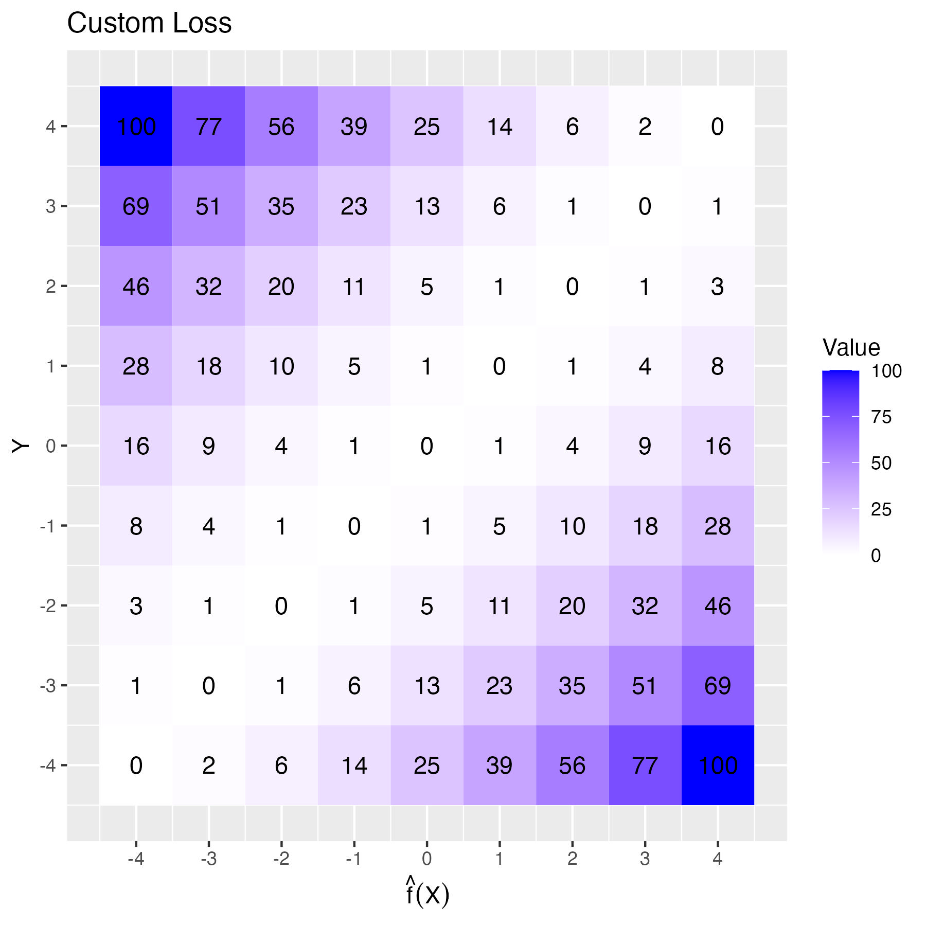
For example, classifying a true y=-1 as -3 “costs” 4, but if you classify it as +1, which is also 2 units apart, it costs +5. That’s the custom “sign error” penalty of the metric.

Ideally, the metric you choose can be used as a loss function, the function that is directly optimized during the training. However, this might not always be possible:

The performance metric might not be differentiable, but, for example, training neural networks requires a loss function with a gradient.
Some model classes have a “built-in” loss function, like the linear regression model which optimizes the squared loss by default, or decision trees that optimize the Gini metric.
The performance metric might not be difficult to optimize because it’s non-convex or infeasible to compute.
The performance metric might only work on an aggregation of your data (e.g. F1 score), but the model requires an instance-wise computable loss function.

Here are some practical tips for working with loss functions and performance metrics:

If possible, design the performance metric so that it’s convex and has a gradient. This way, you can use it directly as a loss function, at least for some model classes such as neural networks.
If you can’t develop the perfect loss function, at least align the loss function with the performance metric: Do they at least have the same optimum? Do they model the same (dis)similarities? Do they both have the same scaling? Think linear versus squared.
Ensure that hyperparameter tuning and model selections are based on the performance metric and not the loss function.
If you have different options for loss functions, you can treat the loss as a hyperparameter.
Even if the loss function optimized by some model class seems like a mismatch, train the model anyway and let the model selection process decide. In the case of a huge mismatch between loss and performance metrics, it should show up in the performance evaluation.

9.4 Considering various evaluation metrics

Supervised machine learning has a drawback: the evaluation is typically based on just one dimension, the performance metric. But life is never that simple! You might have multiple metrics that you care about. And it’s possible to train models that optimize different metrics.

Imagine we want to predict tornadoes in the next hour. We could have accuracy or F1 score as one metric, but there’s more to life than just being right all the time. We might also want to consider the complexity of the model, like how sparse it is, or even the average time it takes to make a prediction (because nobody likes waiting, especially if there’s a tornado looming).

There are two options to accomplish this:

Combine both metrics into one. This only works when you can quantify your desired trade-off between the two metrics.
Use multi-objective optimization for hyperparameter tuning and model selection.

Here are a couple of metrics that you can optimize for, partially based on Pfisterer et al. (2019):

Predictive Performance: Can be quantified using many different measures such as F1-Score, AUC, or mean absolute error.
Interpretability (Molnar, Casalicchio, and Bischl 2020): Metrics such as sparsity, interaction strength, and complexity of the main effects.
Fairness: Measured as disparate impact, equalized odds, or calibration.
Robustness: Measured via performance under perturbations, presence of adversarial examples, and under distribution shifts.
Alignment with physics-based models, for example as in Letzgus and Müller (2023)
Inference time
Memory requirements

Let’s say you want to predict a disease outcome using gene expression data. From domain knowledge, you know that only a few genes might be relevant, but if you only optimize for predictive performance, the model might pick up more genes than necessary if it doesn’t hurt the performance bottom line. By also optimizing for sparsity in this example, you can find a model that satisfies both performance and sparsity¹. We’ve already discussed constraints in a previous section, but multi-objective optimization offers a slightly different approach to constraints. Optimizing for multiple objectives produces multiple “optimal” models. Each model is optimal regarding a different trade-off between the objectives, also known as “Pareto-efficient” models. Having multiple models can be both a bug and a feature. It’s a bug because you typically want just one model. It’s a feature because the set of Pareto efficient models allows you to choose the trade-off between the metrics that make sense based on domain knowledge. And that’s easier than having to decide beforehand how to balance both performance metrics.

Again, we can observe the two-way street: Whether you collapse the objective into one function or you embrace the multiplicity of models with different trade-offs – multi-objective optimization will enable you to explore different trade-offs and therefore feed back domain knowledge.

9.5 Think about inductive biases and learn from them

Inductive bias

The prior assumptions a machine learning algorithm imposes on the model to help generalize to unseen data.

Imagine a machine learning algorithm that produces “models” that only memorize training data. To “predict”, this model would have to check whether the new data point is in the training data. If it is, the model can return the outcome for the training data point. If not, it can’t make a prediction. But what if a training data point is almost identical to the new one? Could we just use the same prediction? The model could then just return the prediction of the nearest data point. Or, to make it robust, the average prediction of multiple close data points from the training data. That’s the idea behind K-nearest neighbors.

But you could also have a model that makes different assumptions about how to generalize to new data, see Figure 9.1. If you get a new data point and one of the features is slightly different from one of the training data points, you could interpolate linearly between the neighboring data points for this new data point. If you do that for all features and training data points, then you end up with a linear regression model.

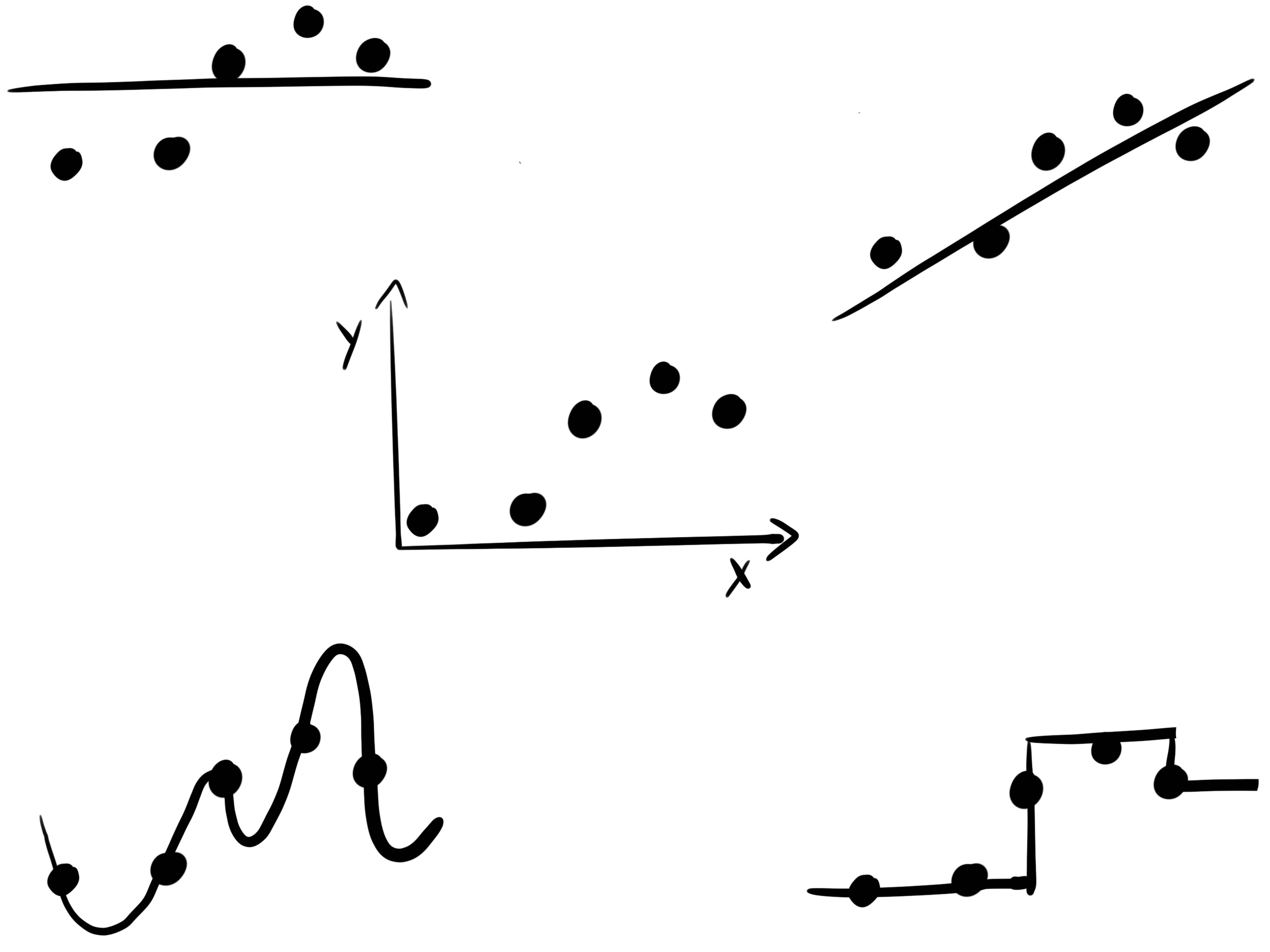
Figure 9.1: Same data, different inductive biases.

Or you could use another strategy: Divide your data into partitions which are defined by binary decisions in the features. The partitions are chosen so that the training data points within have a similar outcome. This comes with a beautiful generalization strategy: For each new data point, we just have to check in which data partition it falls, based on the feature values, and then take the average outcome of all the training data points as a prediction. This is the strategy that decision trees use.

All these examples show that each model class, like trees, k-nearest-neighbors, and linear models, comes with different inductive biases. The inductive bias is an instruction on how to generalize the relation between inputs and outputs to unseen data.

Try out models with different inductive biases. If a certain inductive bias seems to stand out, study how it relates to the studied phenomenon. Can you learn about your problem at hand?

Multi-objective optimization is not the only method to introduce sparsity into your model. Generally, regularization is employed, implying that only models with inherent sparsity, such as LASSO (a sparse linear model), are considered.↩︎