8 Generalization
This book is a work in progress. We are happy to receive your feedback via science-book@christophmolnar.com.
Little does Juan know that his chest X-ray was one of the data points for a pneumonia classifier. He presented with a fever and a bad cough at the emergency room, but it was “just” a bad flu. No pneumonia. The chest X-ray that ruled out pneumonia was labeled as “healthy” and later used to train a machine learning model. The pneumonia classifier is not for our imaginary Juan though, because this ER visit was years ago and the case is closed. While the machine learners don’t care about Juan’s images specifically, they care about cases like Juan’s: Patients coming to the emergency room with symptoms of a lung infection.
That’s the promise of generalization in machine learning: to learn general rules from specific data and apply them to novel data. To generalize from Juan to many. Without generalization, machine learning would just be an inefficient database. But with generalization, machine learning models become useful prediction machines.
In science, generalizing from specific observations to general principles is a fundamental goal. Scientists usually don’t care about specific experiments, surveys, simulations, or studies, but they use them to learn the rules of our world.
This chapter discusses generalization in machine learning and is structured into three parts, each describing generalization with increasing scope.
- Generalize to predict in theory: This is the theory of generalization as it is typically understood in machine learning. It concerns key topics from statistical learning theory, such as empirical risk, the IID assumption, and a discussion of the double descent phenomenon and its relationship to under- and overfitting.
- Generalize to predict in practice: This section describes a more practical idea of generalization. Rarely does the training setup match the application. To generalize the model to the application data requires attention to things like the data-generating process, non-IID scenarios, and distribution shifts.
- Generalize to understand the phenomenon: This type of generalization is often implicitly the goal of scientists. It bridges the gap from ML theory to scientific applications and discusses data representativeness and the data-generating process.
Nuts are a big gamble. Delicious. But difficult to crack. It can take multiple drops from a height to open one. And then you might get a bad one! Or one that wouldn’t open at all. The ravens set out to build a walnut-quality predictor. Every tenth household had to bring random nuts like walnuts and almonds and a supervised machine learning model was trained. The model could almost classify 100% of the training nuts correctly, but accuracy was much worse in production. An investigation revealed: some nuts that were too tough to open and ended up multiple times in the training data. Also, many ravens used it on hazelnuts, which weren’t represented in the data. The raven scientist saw this as a failure of generalization and decided to investigate further.
8.1 Generalize to predict (in theory)
We want our models to work well on the dataset at hand but also on similar data. One language of similarity is that of statistical distributions. You can think of distributions like a huge bucket that contains infinitely many data points. From this bucket, you can draw data and record it. Like the bucket that contains X-rays and their corresponding labels, we denote this bucket by the statistical distribution P(X,Y), where X describes the X-rays and Y the labels. Equipped with distributions, we can describe more elegantly what our models should do.
Machine learning models should be optimal in terms of the expected loss function R(f), also called the expected risk:
\[R(f) = \mathbb{E}_{X,Y}[L(Y, f(X))] \]
It describes the expected error the model will make on instances drawn from the distribution bucket P(X,Y). The “error” for one data point is described by loss function L which quantifies the error between prediction f(x) (e.g. pneumonia) and the actual outcome y (e.g. healthy). The problem is that we don’t know what the bucket – aka distribution – looks like. We only have a limited amount of data that we recorded. When we have data, we look at the errors the model makes on these data and average over it.
You could use the training data to estimate the expected loss, but using training data makes for a bad estimator of R(F). The estimated loss would be over-optimistic, meaning too small. If a model overfits the training data (“memorizing” it), the training error can be low even though the model won’t work well for new data. It’s like preparing students for an exam by giving them the exam plus the perfect answers and then testing them on the exact same exam – you won’t get an honest assessment of the student’s skills on the subject. The X-ray classifier might work perfectly for Juan and the other training data subjects, but not for new patients. But this has a simple solution: Estimate the expected risk using new data.
\[\hat{R}(f) = \sum_{i=1}^{n_{test}} L(y^{(i)}, f(x^{(i)}))\]
This formula is also known as test error, out-of-sample error, generalization error, or empirical risk (on the test set). Slowly but finally, we are getting somewhere – a language to talk about generalization. A model generalizes well when \(\hat{R}(f)\) is low and when the so-called generalization gap is small, which is defined as the difference (Hardt and Recht 2022):
\[\delta_{gen}(f) = R(f) - \hat{R}(f)\]
If the generalization gap is small, the model will perform similarly well for training and unseen data. Confusingly, the generalization gap is sometimes referred to as the generalization error. Let’s explore how the generalization error behaves in different scenarios.
Underfitting and Overfitting
Machine learning can feel more like an art than a science, but we have an entire field dedicated to putting all the deep learning magic and mystical random forests on a scientific grounding: statistical learning theory, which provides a view on machine learning from a statistical lens. We explore some concepts from statistical learning theory to shed some light on generalization.
One well-known and well-studied concept is overfitting and its counterpart, underfitting. Underfitting is when the model is not complex enough to model the relation between input and output, so the model will have both a high training and test error but a small generalization gap. Underfitting models are, frankly, bad! Overfitting is when the model function has a bit too much freedom: It fails to capture generalizable rules and instead “memorizes” the training data. That’s why overfitting is characterized by a low training error, but a high test error and therefore a large generalization gap. Both underfitting and overfitting are undesirable as they both mean a failure to generalize well (measured as low out-of-sample error).
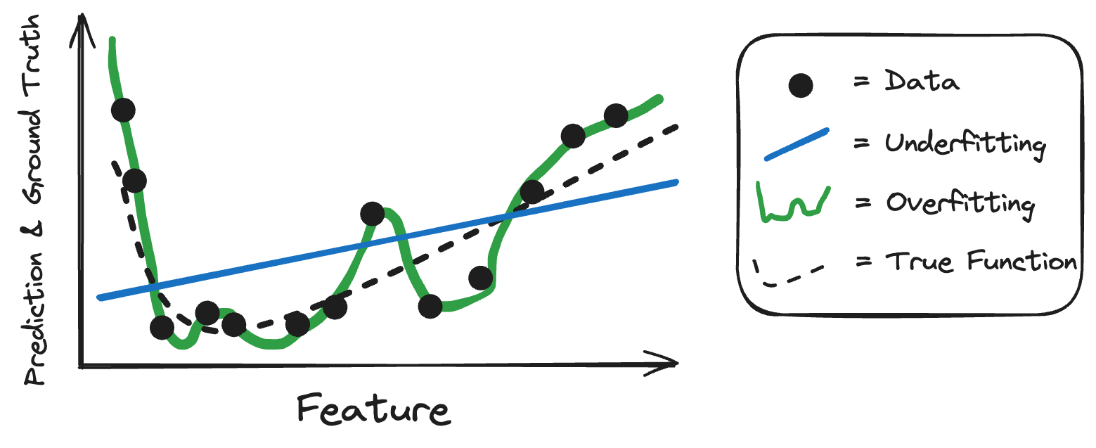
Going back to the chest X-ray example: Imagine the classification algorithm would be a simple logistic regression classifier based on the average grey scale value of parts of the image. It might work better than random guessing, but wouldn’t produce a useful model. A case of underfitting. Overfitting in this same case would look like this: Let’s say we use for the chest X-ray a decision tree that is allowed to be grown to full depth. Inputs are the individual pixels and all typical restrictions are lifted, like having a minimum amount of data in each leaf. The tree could grow very deep and separate all training data, uniquely identifying them. But when used on new data, the decision tree would fail. Figure 8.1 showcases underfitting and overfitting on a simple 1-dimensional case.
Whether a model will underfit or overfit depends on the machine learning algorithm responsible and the complexity of functions it can produce. By picking certain types of model classes and their hyperparameters, we can steer the flexibility of the models and therefore the balance between underfitting and overfitting. The typical approach in machine learning is to use fairly flexible models and then regularize them.
Examples of such flexible models are neural networks and decision trees. Theorems show that both neural networks (Cybenko 1989, hornik1991approximation) and decision trees (understood as simple functions) can approximate arbitrary continuous functions (Halmos 2013). These flexible models can then be regularized by specifying certain hyperparameters in modeling such as the learning rate, the architecture, the loss function, or enabling dropout (Goodfellow, Bengio, and Courville 2016).
Underfitting and overfitting don’t tell us about the types of errors the models make. This will be covered in Chapter 12.
8.1.1 Double descent or why deep learning works
We’ve painted a neat picture of what a perfectly balanced model looks like – models should be flexible enough not to underfit and regularized enough not to overfit. But now we have deep learning and the over- and underfitting reasoning doesn’t seem to work any longer. Deep neural networks have millions or more parameters and can perfectly fit the training data in infinitely many ways, so we would expect strong overfitting. The thing is – they generalize. It’s like in society: the laws of under and overfitting developed for the average John Doe model don’t apply to the fancy models rich in parameters. This surprising learning behavior in deep neural networks has been named double descent (Belkin et al. 2019). Double descent describes the out-of-sample error when increasing the ratio between parameters and data. The behavior can be sliced into two components:
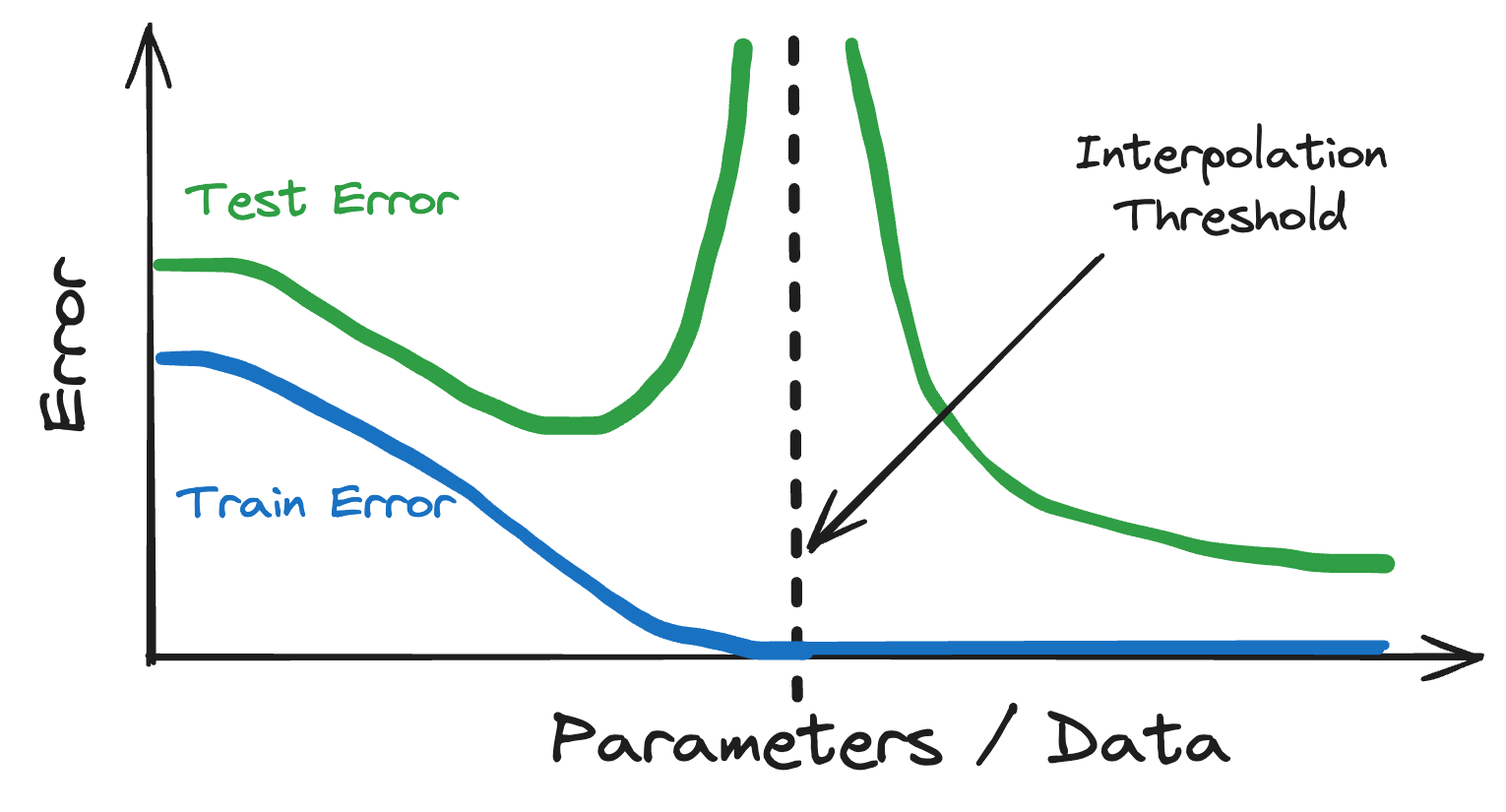
- Typical under- and overfitting: The dataset remains fixed and we start with a simple neural network. If we increase the number of parameters in our model and fit it to the data, we observe the typical underfitting and overfitting. This is true until we reach the point where we have as many parameters as we have datapoints, the so-called interpolation threshold. As expected, the test error explodes when reaching the interpolation threshold.
- Double descent: But unlike traditional under- and overfitting, the test error decreases if we increase the number of parameters beyond the interpolation threshold. Continuing to increase the network size, the test error may even be lower than the test error of the “ideal” model in the underfitting/overfitting world (see Figure 8.2).
Double descent is not exclusive to deep neural networks but also happens for simple linear models (Schaeffer et al. 2023), random forests, and decision trees, as suggested by Belkin et al. (2019), possibly due to a shared inductive bias. Double descent undermined the theory of underfitting versus overfitting. But under- and overfitting are still useful concepts. It’s like with Newton’s theory of gravity when Einstein’s relativity came along: Underfitting and overfitting provide an accurate picture of things below the interpolation threshold, but beyond this threshold the classical picture becomes invalid.
Double descent describes the what but not the why. We still have no definitive answers as to why overparameterization works so well, but there are theories:
- The lottery ticket hypothesis (Frankle and Carbin 2019) says that there are subnetworks in certain trained neural networks that have similar performance to the overall network. Training a large network is like having multiple lottery tickets (aka subnetworks) and one will win.
- Benign overfitting (Bartlett et al. 2020): Many low-variance directions in parameter space are required to achieve highly performing models. This is achieved through overparameterization and makes for “benign overfitting”.
- Implicit regularization (Smith et al. 2020): Optimization algorithms such as stochastic gradient descent implicitly regularize the model. It was shown that stochastic gradient descent actually optimizes not only the loss but effectively the loss plus an implicit minimizer.
We barely scratched the surface of statistical learning theory, and there are many more topics to explore:
- Quantifying the complexity of models (like VC dimensions)
- Providing a priori learning guaratees for kernel methods (like support vector machines)
- Studying consistency and convergence rates of learners
- Bounding the empirical risk
8.2 Generalize to predict (in practice)
So far we’ve talked about generalization from a theoretical viewpoint that, in practice, is too narrow. In practice, we only have access to data not to the underlying distributions. And even this data is messy, noisy, and cannot perfectly be trusted.
Generalization through splitting data
Let’s say, as is so often the case in practice, data is in scarce supply. How to obtain models that generalize while being data-efficient? The answer – smart data splitting! Let’s explore this with an example: Rajpurkar et al. (2017) built a chest X-ray image classifier to detect pneumonia. To ensure that the classifier generalizes to new data, they split the data into training data (93.6% of the data), validation data (6%) to control the learning rate, and test data (0.4%) to evaluate the final model. If they had used 100% of the data for training the model, they would run into two problems: 1) It might perform badly since it’s unclear for how many epochs to train the model, and 2) the modelers would have no idea about the performance of the model, except for an overly optimistic estimate on training data.
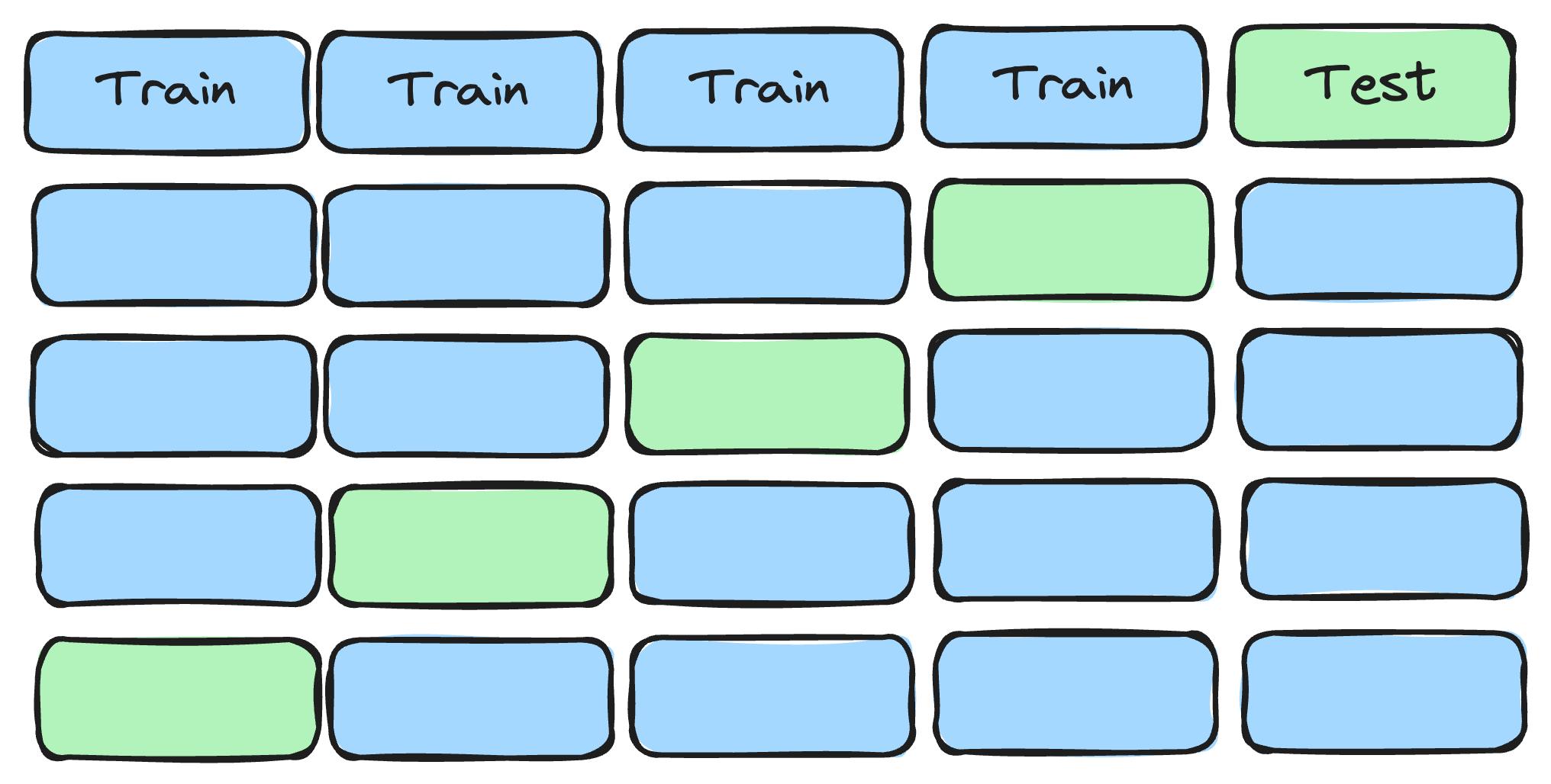
But if you split the data, train a model on one part, and evaluate the model on the remaining part, you can get an honest estimate of the out-of-sample error. Great, problem solved?! Careful, while their approach gets them an unbiased estimate of the test error, the estimate possibly has a large variance. With only 420 images in the test set, 10 difficult cases that ended up in the test set by chance can spoil your performance estimate. One strategy to lower the variance is to split the data more often. For example with cross-validation: Split the data, for example, into 5 parts, combine 4 parts for training (and validation), and the remaining 1 part for testing. Repeat this setup 5 times so each part is once used as test data. Average the 5 estimates of the out-of-sample error and, voila, you have a more stable estimate (visualized in Figure 8.3).
But there’s another problem. In each CV-loop, we split the data once into training and validation data. The validation data in Rajpurkar et al. (2017) was used for adapting the learning rate, but you could also use it for hyperparameter tuning and model selection. A single split can lead to a similar problem as before: too much variance. So you might want to have another cross-validation inside the outer cross-validation. This so-called nested cross-validation quickly blows up the number of models you have to train, but it is a more efficient use of your data.
We quickly went from splitting the data into two parts (training and testing) to splitting the data 100 times (10-fold cross-validation within 10-fold cross-validation). Data splitting is at the heart of generalization.
The tricky IID assumption
Statistical theory and data splitting practices rest on a crucial assumption: data are IID. The term IID stands for “independent and identically distributed” and means that each data point is a random sample:
- Identically distributed: All the data points are from the same distribution and don’t change over time. If you had one set of X-ray data for model training from a children’s hospital but the model application from an adult hospital, they are not identically distributed.
- Independent: A data point doesn’t reveal the ground truth of another data point. The X-ray data are no longer independent if a patient appears multiple times. Sampling one X-ray of a patient reveals information about other X-rays of the same patient.
IID is a typical assumption in statistical learning theory, but also when we randomly split data for generalization purposes we implicitly have this assumption. IID is restrictive and real-world data often violates it. Some examples:
- Store sales over time are not IID.
- Patient visits with possibly multiple visits per patient are not IID
- Satellite images of neighboring locations are not IID.
An earlier version of the paper by Rajpurkar et al. (2017) ran into this non-IID problem: They split the data randomly, but for some patients, there were multiple X-ray images in the data. This led to data leakage: The model had an easier job since the model was able to overfit patient characteristics (e.g. scars in the X-ray image) and that would help classify the “unseen” data. As a kid, our imaginary Juan fell from a tree and broke his rips. This past injury is still visible in chest X-ray images and uniquely identifies Juan. If Juan went multiple times to the emergency room, his images might end up in both training and testing.
Rajpurkar et al. (2017) fixed this problem by ensuring that a patient’s data can only be in training or testing, but not both. If IID is violated, generalization can break down in parts – unless we account for it. The IID assumption also helps us in estimating the test error: If the data are IID, we can estimate the generalization error in an unbiased way because of the law of large numbers.
The real world is messy
When COVID hit, many machine learning research labs dropped their projects to work on COVID detectors, many of them from X-ray images. Partially understandable, but in hindsight, a waste of effort. Sounds harsh, but Wynants et al. (2020) did a systematic review of 232 prediction models for COVID and found that only 2 (!) were promising. The remaining 230 had various problems, like non-representative selections of control patients, excluding patients with no event, risk of overfitting, unclear reporting, and lack of descriptions of the target population and care setting.
If you want a functional COVID-19 X-ray classifier, you should be as close as possible to the data-generating process of a potential application. For instance, getting data directly from an ER where radiologists label the images with the diagnoses. This would generate a dataset that reflects a typical distribution of cases. However, the data that many ML labs used were quite different. So different that the research models and results are unusable. As the pandemic progressed, more and more X-ray images of COVID-ridden lungs were posted online in repositories. Often without metadata (e.g., missing demographics of the patient), without any verification process, and little documentation. But that’s not the worst part of COVID classifiers. For classification tasks, you also need negative examples, such as images of healthy lungs or from patients with, for example, pneumonia. Instead, the negative images were cobbled together from many pre-pandemic datasets. A red flag: Negative and positive X-ray data come from different datasets. Should a deep learning model find any hints or shortcuts that identify the data source, then it doesn’t have to identify COVID at all. But even that isn’t the worst yet. The worst is how the non-COVID dataset was assembled. Roberts et al. (2021) looked more deeply into the most commonly used datasets and found the following fouls:
- The X-ray image datasets were put together from multiple other image datasets.
- One of these datasets was from children (only non-COVID).
- Some datasets were included more than once, leading to duplicated images, introducing non-IID problems and data leakage.
- For some of the datasets it’s intransparent how they were collected
- Other datasets were collected through “open calls” to other researchers to submit data without further verification.
These things should all raise red flags. It’s like Frankenstein was employed to generate a dataset. A data-generating process that deviates strongly from any application we can think of. A model trained on Frankenstein’s data can learn all matters of shortcuts and none will generalize to a meaningful application:
- Identify children’s lungs: if the model can identify that the image was from a child, it can safely predict “not COVID”.
- Identify the year: If the model can identify the year through explicit or implicit markers (like the type of machine) it can safely label “not COVID” for older images.
- Identify the dataset: Any characteristics that images from the same dataset share can be used to make the prediction task easier. It’s enough when a dataset was processed differently (e.g. greyscaling) or comes from a different X-ray machine.
- Duplicates: Some images might have ended up both in training and test data, making the model seem to work better than it does.
Even if you find a model that perfectly predicts identically distributed data, the models can’t be used. No application comes with a data distribution anywhere identical to this mess.
In general, to generalize from training to application, you want the data-generating process to look as similar as possible. It’s difficult. The world is even messier than what we described here and there are many more challenges to generalization in practice:
- Distribution Shifts: Imagine someone building a pneumonia classifier before COVID-19. COVID introduced a new type of pneumonia and due to lockdowns and social distancing other types of pneumonia occurred less frequently. A massive distribution shift may worsen the performance of existing models. Distribution shifts are discussed in Chapter 13.
- Non-causal models: The more a model relies on associations but not causes, the worse it might generalize. See Chapter 11.
- Using an unsuitable evaluation metric: While this may not show up in a low test error, picking a metric that doesn’t reflect the application task well will result in a model that transfers poorly to the real-world setting.
8.3 Generalization to understand a phenomenon
Generalization to predict other data is one thing, but especially in science we often want to generalize insights from the model to the phenomenon we are studying. In more statistical terms this is about generalizing from a data sample to a larger population. A theme that is less spoken about in machine learning, but something we have to talk about.
Generalization of insights may even come in innocent ways that we don’t immediately recognize. For example, Rajpurkar et al. (2017) claimed that their X-ray classifier performs on par with radiologists, even outperforming them on certain metrics. We could say they only refer to the test data and leave it at that. But nobody is interested in the test data, but in the population they represent. Like a sample of X-rays taken typically in the emergency room. Unfortunately, the paper doesn’t define the population, which is typical for machine learning papers.
If a researcher studies a phenomenon, say, the effect of fertilizer on almond yield (like Zhang et al. (2019)), using machine learning and interpretability techniques, they also generalize. They generalize, explicitly or implicitly, from their model and data to a larger context. Quoting from the abstract of Zhang et al. (2019):
We also identified several key determinants of yield based on the modeling results. Almond yield increased dramatically with the orchard age until about 7 years old in general, and the higher long-term mean maximum temperature during April–June enhanced the yield in the southern orchards, while a larger amount of precipitation in March reduced the yield, especially in northern orchards.
The larger context depends on what the data represents. In the case of the fertilizer study, this might be all the over 6,000 (“The California Almond” n.d.) orchards in California. Or maybe it’s just the ones in Central Valley? It depends on how representative the dataset is. The word representativeness or especially representative data is overloaded and people use it differently in ML (Clemmensen and Kjærsgaard 2023) and science (Chasalow and Levy 2021). In the broadest sense, “representativeness concerns the ability of one thing to stand for another—a sample for a population, an instance for a category” (Chasalow and Levy 2021). In machine learning some claim representativeness without argument, some claim non-representative because of selection biases, some mean that the sample is a random sample from the distribution, and some claim coverage in the sense that all relevant groups are covered (maybe not in the same frequency as target population though), some speak of it as prototypes and archetypes. But for science and especially for the goal of inference – to draw conclusions about the real world – we need the data to represent the target population, in the sense of the training data being a random sample from the population.
In an ideal world, you start with your research question and define the population about which the question is. Then you draw a perfectly representative sample because you can just randomly sample from the population, as easy as buying fresh bread in Germany. But that’s often far from reality. The other way would be to start with a dataset, argue which population it represents, and extend insights to this population. And sometimes it’s a mixture of bottom-up and top-down approaches. Zhang et al. (2019), for example, describes that they collected data from the 8 major growers that make up 185 orchards in the Central Valley of California. Some in the northern, some in the central, and some in the southern region. However, they do not discuss whether their sample of orchards is representative, so it’s unclear what to make of the results.
Proving that your data is representative is difficult to impossible. If you know the population statistics, you can at least compare summary statistics between the training set and the population. As always, it’s easier to disprove something: finding a single counter-argument is enough. For representativeness, the counter-arguments are called “selection biases”. Selection biases are like forces in your collection process that either exclude or at least undersample some groups or over-emphasize others. Selection bias is a good angle to view the collection process. If you have identified a selection bias, you can discuss its severity and maybe even counter it by weighting your samples. Some examples of selection biases include:
- Survivorship bias: The sample only includes “survivors” or those whose objects/subjects passed a selection process.
- Non-response bias: Human respondents can differ in meaningful ways from non-respondents.
- Exclusion bias: Some exclusion mechanism (e.g., due to missing data) biases the sample.
8.4 No free lunch in generalization, and no free dessert either
We structured this chapter along three types of generalization: to predict in theory, to predict in practice, and to understand a phenomenon. One of the most well-known theoretical results – the so-called no-free lunch theorems – has taught us that generalization never comes for free (Wolpert 1996). All versions of the theorems highlight the following: We will never attain an ultimate learning algorithm that just fed with data always spits out the best possible prediction model (Shalev-Shwartz and Ben-David 2014). We must take an inductive leap to generalize from a data sample to anything beyond itself. Like making context-specific assumptions (e.g. smoothness or IID) (Sterkenburg and Grünwald 2021). There ain’t no such thing as a free lunch, if you want to eat different meals, you need different cooking recipes.
And, unfortunately, there is no free dessert either. Even if we have a model that generalizes well to identically distributed data, we have to “pay” for any further generalization. When it comes to generalization from training to application or from sample to population, we need to make even more assumptions and put in extra effort. And sometimes we might not achieve them after all. Generalization is never free.
The cost of generalization comes up in other chapters as well:
- When interpreting the model for the goal of understanding the phenomenon of interest, we make assumptions about representativeness for example (see also Chapter 10)
- For causal inference, we make assumptions about the causal structures in the world (Chapter 11)
- The topic of fairness also requires us to look into generalization from an ethical perspective (Chapter 14)
- Robustness is about guarding our models against distribution shifts (Chapter 13)