10 Causality
Machine learning exploits all available information to make predictions – and there are many ways to predict things. A good example of this is assessing a person’s COVID risk. You can predict it from features such as:
- wearing a mask
- symptoms like dry cough
- vitamin D levels
From a causal perspective, these features relate differently to the COVID risk. This difference is illustrated in the so-called causal graph below, which is a graphical tool for thinking about causal dependencies.
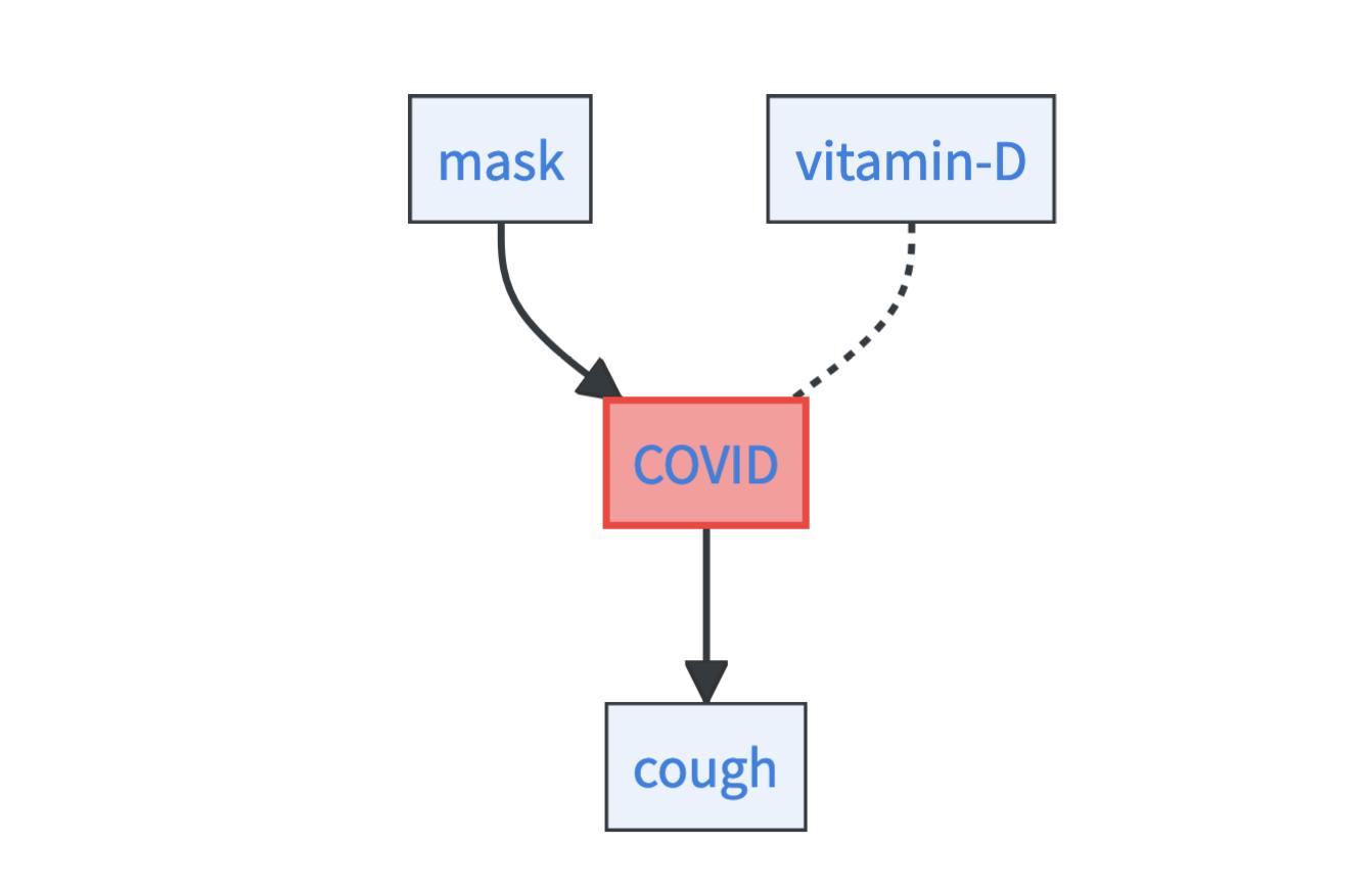
- Causes: Wearing a mask is a causal factor for the COVID risk. Why is it a cause? Well, those who put on a mask can thereby lower their COVID risk [1]. The fact that masks are causal for COVID risk is highlighted by the outgoing arrow from the mask node to the COVID node.
- Effects: Dry cough is an effect of COVID [2]. People who are healthy and then get infected with COVID likely get dry cough as a symptom. Importantly, it is not a cause of COVID – if people take cough sirup this may help against their cough but does not change their COVID risk. The fact that dry coughing is an effect of COVID is highlighted by the incoming arrow to the cough node from the COVID node.
- Associations: Vitamin D levels are associated with COVID risk [3]. For example, in the overall population, people with higher vitamin D levels less often get COVID than people with low vitamin D levels. Still, it is unclear if higher vitamin D levels cause a lower COVID risk or if the association arises for entirely different reasons. The unexplained association between vitamin D levels and COVID is highlighted by an undirected dashed arrow.1
Initially, there was a lot of hype about machine learning in Raven Medicine. Some even proclaimed the end of costly medical experiments. But the enthusiasm soon waned: Machine learning provided little insight into how to treat Ravens to make them healthy. Was the red pill or the blue pill more effective? The old proverb “correlation is not causation” hit the machine learning enthusiasts hard.

10.1 Prediction does not require causal understanding
All the features we have just listed can be equally helpful in predicting COVID risk with machine learning. You may decide to rely only on causes or only on effects:
- Predict effects from causes: An example is the protein folding problem discussed at the beginning, where the amino acid sequence causally determines the protein structure [5].
- Predict causes from effects: An example is predicting the presence of a black hole from its gravitational effects on the surrounding bodies.
- Mixed prediction: This is probably the most common case. An example is medical diagnosis. To diagnose malaria, doctors take into account symptoms like high fever but at the same time causes such as a mosquito bite from your South America travels.
In the end, it is your decision as a modeler what you want to incorporate in your prediction model, whether it is causes, effects, causes of effects, or even spurious associations. For the machine learning model to successfully predict, all that matters is that the feature contains information about the target variable.
10.2 Costly experiments distinguish causes from effects
Controlled experiments are the best approach to distinguish between causes and effects. Let’s say you have two variables, vitamin D and COVID. To establish whether higher vitamin D levels reduce the COVID risk, you could run a randomized control trial (RCT). You have 10,000 test subjects: 5,000 randomly selected subjects belong to the treatment group (they get vitamin D supplements); the other 5,000 belong to the control group (they get placebos). If after a certain time, the COVID infections in the treatment group are significantly lower than in the control group, you can conclude that vitamin D is a causal factor for COVID risk. Easy, right?!
Unfortunately, conducting controlled experiments in the real world is cumbersome. It takes a lot of time, money, and resources. Some experiments can be ethically or legally problematic, such as the administration of harmful drugs to humans. Other experiments are beyond the capabilities of humans – like investigating the effects of pushing Jupiter out of its solar trajectory – you’d need to be as strong as Saitama 2 for that…
Social scientists, in particular, often deal with observational data. Observational data is data that is measured without controlled conditions. Like asking random people on the streets for their vitamin D levels and if they had COVID. Observational data is what we gather all the time – the little measuring device in your pocket is piling up tons of it.
10.3 Machine learning can generate causal insights
Observational data is what you are likely feeding your machine learning algorithm. Unfortunately, observational data alone does not provide causal insight [6].
It is impossible to distinguish causes from effects from observational data alone [6].
If you cannot even distinguish between causes and effects from observational data alone, how can machine learning help with causality? It turns out that machine learning can help with causal inference (answering causal questions with the help of data), but usually not for free: You have to make assumptions about causal structures.
These are the causal questions that machine learning can help with:
- Studying associations to form causal hypotheses: Machine learning helps to investigate associations in data such as the association between COVID and vitamin D levels, which can be the starting point for causal hypothesizing.
- Estimating causal effects: Machine learning can be used to estimate causal effects, such as quantifying the effect of vitamin D on the COVID risk.
- Learning causal models: You can use machine learning to learn causal models. Causal models are formal tools to reason about real-world interventions and counterfactual scenarios.
- Learning causal graphs: Causal graphs encode the direction of causal relationships, and machine learning can help learn them directly from data.
- Learning causal representations: Machine learning can learn causal variables, which are high-level representations (e.g. objects) of low-level inputs (e.g. pixels).
These five tasks structure the rest of this chapter.
10.4 Studying associations to form causal hypotheses
You may have heard that machine learning models are capturing complex associations in data. But what are associations? It is easiest to understand associations by their opposite, namely statistical independence. Two events are independent if knowing one event is uninformative about the other, e.g. knowing about your COVID risk does not tell anything about the weather on the planet Venus. More formally, two features \(A\) and \(B\) are statistically independent if \(\mathbb{P}(A\mid B)=\mathbb{P}(A)\). We call two features associated whenever they are not statistically independent. For example, COVID risk is associated with wealth. Statistically, the higher your wealth the lower your COVID risk [7]. But be careful, associations are complex creatures. For example, wealthier venders are likely to have a higher COVID risk than poor venders because they have contact with more customers. This is called an interaction effect.
Like classical statistical techniques, machine learning together with interpretability methods (see Chapter 9) enables you to read out complex properties of your data. You can for example study:
- Feature effects & interactions: How is the target associated with certain input features?
- Feature importance: How much do certain features contribute to the prediction of the target?
- Attention: What features is our model listening to when predicting the target?
10.4.1 Form causal hypotheses with the Reichenbach principle
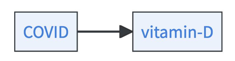
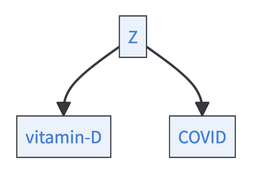
Assume you find in your data the association between vitamin D and the COVID risk. Then, the Reichenbach principle can guide you in forming a causal hypothesis. The principle states three possibilities where the association can come from [8]:
- Vitamin D can be a cause of COVID.

- COVID can be a cause of vitamin D.
- Or, there is a common cause \(Z\) of both, vitamin D and COVID.
Nothing against Reichenbach, but in reality, there are two more explanations for the association:
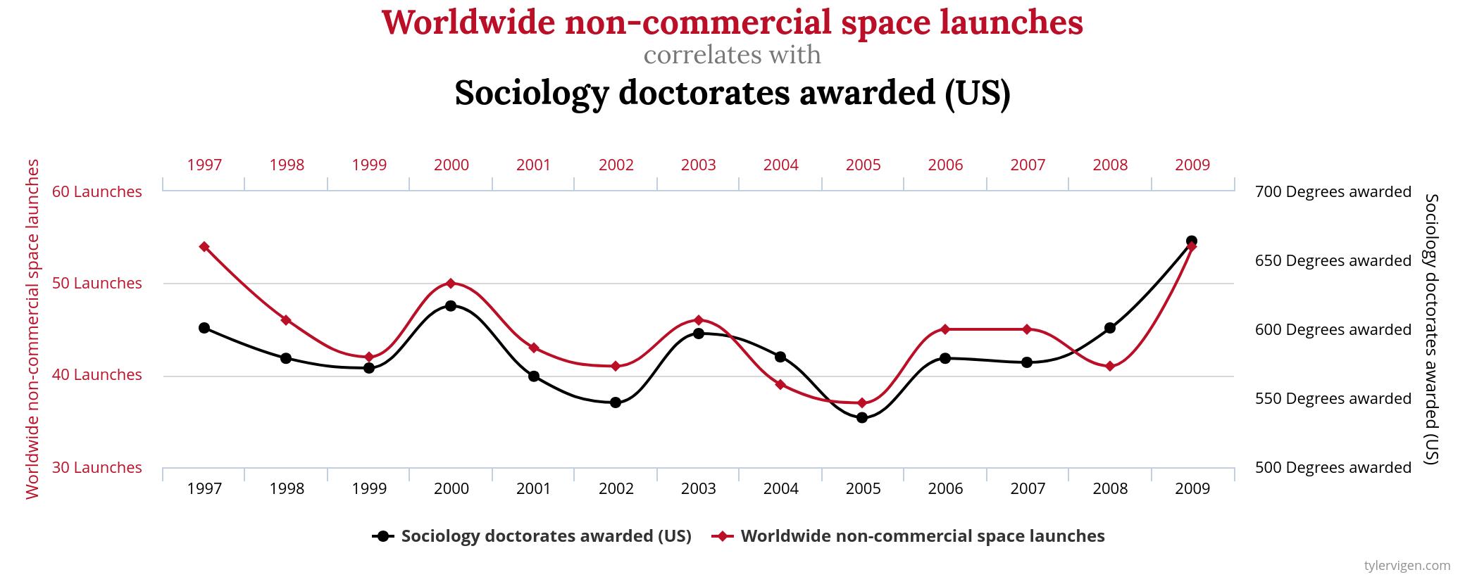
- First, the association can be spurious. It is only there because of limited data. If you continue gathering data, the association will vanish. Figure 10.1 shows an almost perfect association between worldwide non-commercial space launches and the number of doctorates awarded in sociology [9]. But is it causal? Perhaps Elon Musk can boost his business by awarding a few PhD scholarships in sociology…
- Second, the association can result from a selection bias in the data collection process. It occurs if the data sample is not representative of the overall population. For example, while niceness and handsomeness are probably statistically independent traits in the overall population, they can become dependent if you only look at people you would date [10].
But how to identify the correct explanation for the association between COVID and vitamin D? Because there is a lot of data (not spurious) and the association is found in the overall population (no selection bias), you may infer that one of Reichenbach’s three cases applies. Gibbons et al. [11] compared a large group of veterans receiving different vitamin D supplementations to a group without treatment. They found that the treatment with vitamin D reduces the risk of getting COVID significantly and therefore recommend broad supplementation. Even though the study was not a randomized control trial, it strongly indicates that there is a causal link between vitamin D levels and COVID risk.
The scientific story may continue at that point: There might be unknown common causes of both vitamin D and COVID risk. Moreover, the causal link does not explain by what mechanism in the body vitamin D acts on COVID risk. That’s how science works, new questions keep popping up…
10.4.2 Select explanatory variables with feature importance
Importances of features primarily allow you to evaluate which features are most informative for predicting the target. For example, they may tell you whether vitamin D levels contain any information about your COVID risk beyond the information that is already contained in the mask and the cough features. But importance itself gives no causal insight. It can still be useful for a causal analysis: importance allows you to understand what information is redundant, noisy, or just unnecessary. This may prove helpful in selecting sparse and robust features for a causal analysis [12].
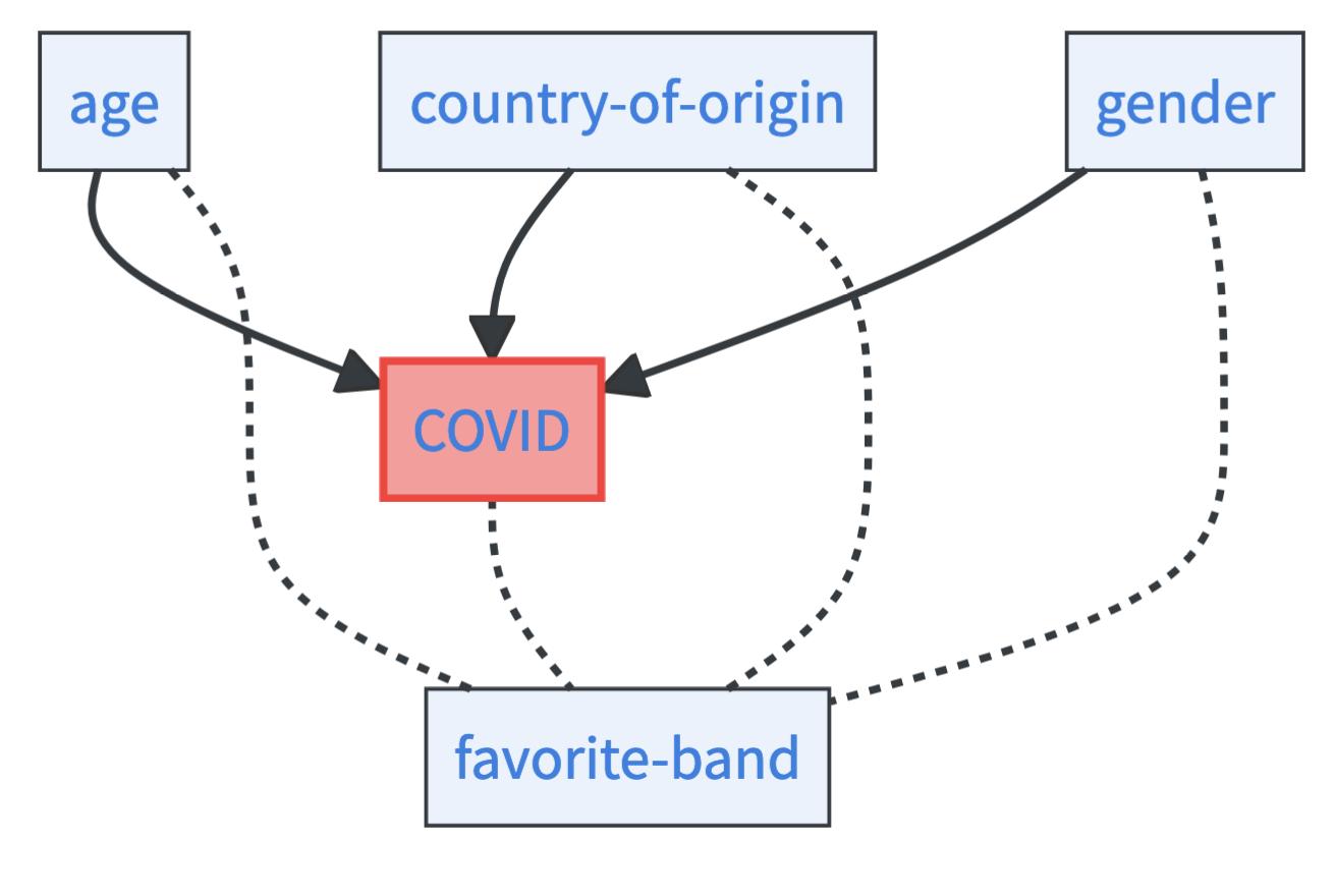
Imagine you know a person’s age, country of origin, gender, favorite color, and favorite band. You want to predict again her COVID risk. By studying feature importance, you may find out that:
- The favorite color has very little importance under all constellations. It might even have negative importance as it introduces noise.
- The favorite band is extremely informative. You can even drop all other features without a major loss in predictive performance.
- If you know the age, country of origin, and gender of a person, knowing her favorite band does not add much.
Depending on your goal, this can be very insightful. You can generally drop the favorite color feature, it is not predictive and will not provide insights for a causal analysis. If you want to reason about policy interventions to lower the COVID risk, you can exclude the favorite band from your causal analysis. If, on the other hand, you are a sociologist who wants to study how taste in music is related to health, you may want to keep all features.
10.4.3 Find high-level variables with attention
The question of what a model is attending to in its decisions is prominent in interpretability research, particularly in image classification [13]. Although scientists may be more concerned with the relationship in the data than in the model, model attention may still be relevant if the input features have meaning only in the aggregate, not individually. Think of pixels that constitute images, letters that constitute sentences, or frequencies that constitute sounds. Attention can point you to meaningful constructs or subparts that are associated with the target and allow you to form causal hypotheses about them.
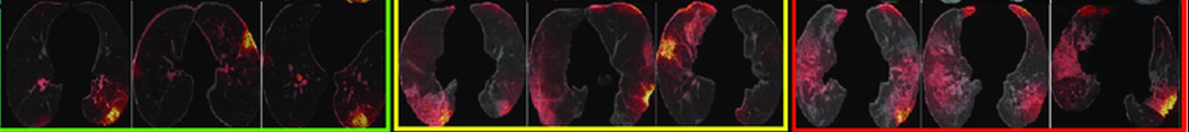
For example, while predicting COVID from CT scans sounds like taking a sledgehammer to crack a nut, it can be an interesting approach to learning more about how the disease affects the human body. Even though the input features themselves are pixels, they collectively form higher-level concepts that can be highlighted by saliency-based interpretability techniques. This approach was for example used by [14] to detect lesions in the lungs of COVID patients as illustrated in Figure 10.2.
10.5 Estimating causal effects with machine learning
So far, we have assumed that researchers are searching in the dark, where they use machine learning to find interesting associations to form and test causal hypotheses. However, often researchers have causal knowledge or intuitions about how features relate to each other. Their goal is causal inference, or, to be more precise, to estimate causal effects, which is a more well-defined problem than just exploring associations.
Causal graphs show causal dependencies, e.g. if you put on a mask, it will causally affect your COVID risk. But this begs the question of how it affects your risk. Is wearing a mask lowering your COVID risk and if yes, by how much? This question asks for a causal effect. Questions for causal effects were omnipresent during the pandemic:
- How does vaccination affect the COVID risk of elderly people?
- How does the average COVID risk change with contact restrictions compared to without them?
- How does treatment with vitamin D pills lower the COVID risk of African Americans [11]?
Causal effects always have the same form. You compare a variable of interest such as COVID risk with treatment, for example, masks, against those without treatment (no-mask). This gives us the so-called Average Treatment Effect (ATE). In the case of masks being the treatment, we can formally describe the effect on the COVID risk:
\[\text{ATE}=\mathbb{E}[\text{COVID}\mid do(\text{mask}=1)] - \mathbb{E}[\text{COVID}\mid do(\text{mask}=0)]\]
Let’s unpack this formula. The do in the ATE denotes the do-operator, which means you intervene on a variable and set it to a certain value. Thus, the first term describes the expected COVID risk if you force people to wear masks. The second term describes the expected COVID risk if you force people not to wear masks. The difference between the two terms describes the causal effect of masks on the COVID risk.
In many cases, rather than asking for the ATE, you ask for the treatment effect for a specific subgroup of people that share certain characteristics. During the pandemic, for example, researchers might have asked about the causal effect of masks for children under 10 years of age. This is the so-called Conditional Average Treatment Effect (CATE):
\[\begin{align*} \text{CATE} &= \mathbb{E}[\text{COVID} \mid do(\text{mask}=1), \text{age}<10] \\ &\quad - \mathbb{E}[\text{COVID} \mid do(\text{mask}=0), \text{age}<10] \end{align*}\]
The do() terms in the two formulas give the impression that you have to run controlled experiments to estimate the causal effects. And conducting experiments would be the most reliable way – if you can do it, you should! Unfortunately, experiments are sometimes not feasible. In some situations, you are lucky because you can estimate the ATE and CATE from observational data alone. If this is the case, the causal effect is identifiable.
10.5.1 Identify causal effects with the backdoor criterion
The classical way to identify a causal effect is via the so-called backdoor criterion. The idea is simple. Let’s say you want to know the ATE of masks on the COVID risk. You only have observational data. But your data allows you to read out: 1. how many people with masks got infected and 2. how many people without masks got infected. Just subtract the latter from the former and you are finished, right? No! The problem is that the information you want to obtain is potentially blurred by other factors. For example:
- Sticking to the rules: People who stick to the rules are more likely to wear masks and also follow other rules like contact restrictions. Therefore, they also have on average a lower COVID risk.
- Number of contacts: People who have many contacts (e.g. postmen, salespeople, or doctors) wear masks to lower their own risk and the COVID risk of others. But many contacts increase also their COVID risk.
- Age: Younger people are less likely to wear masks because they think masks do not look cool or because COVID is less dangerous for young people. At the same time, young people are more resistant to getting infected with COVID [15].
Those factors are called confounders. They are both a cause of the treatment and the variable of interest. Imagine you knew all those confounders and accounted for them. Then, you could isolate the association that is solely due to the masks themselves. This is exactly what the backdoor criterion is doing. If you know all confounders \(W\), the ATE can be estimated by:
\[\begin{align*} \text{ATE} &= \mathbb{E}_W[\mathbb{E}_{\text{COVID}\mid W}[\text{COVID} \mid \text{mask}=1, W]] \\ &\quad - \mathbb{E}_W[\mathbb{E}_{\text{COVID} \mid W}[\text{COVID} \mid \text{mask}=0, W]] \end{align*}\]
A great success, there are no do-terms left. But be aware that knowledge of all confounders is a super strong requirement that can rarely ever be met in reality. And not knowing a confounder may bias your estimate significantly. The same happens if you mistake a variable for a confounder that is caused by both the treatment and the variable of interest (this is called a collider bias). So conditioning on more features is not always better.
The back-door criterion is not the only option to identify causal effects. There is for example also its friendly sibling, the frontdoor criterion. Both, the front and the backdoor criterion are special cases of the do-calculus. Whenever it is possible to identify a causal effect, you can do so using the do-calculus. This book will stay at this surface level on the question of identifiability, if you like math and want to dig deeper, check out [16]. The cool thing is, you don’t have to know all of that necessarily to do causal analysis. The identification step can be fully automated given a causal graph, for example, using the Python package DoWhy [17].
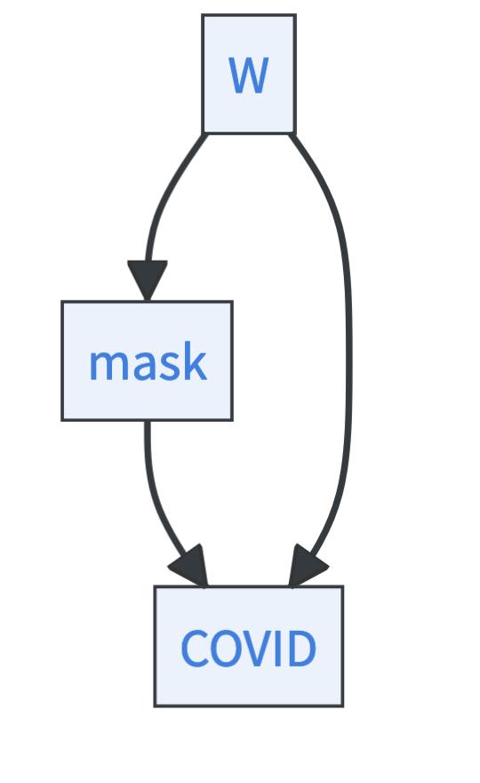
Let’s take a look into two machine learning-based methods that allow for estimating causal effects: the T-Learner and Double Machine Learning 3. Both are designed for the backdoor criterion setting. That means, in both cases, you assume that you have observed all confounders \(W\), and your causal graph looks like this
10.5.2 How to estimate causal effects with the T-Learner
The T-Learner is maybe the simplest approach to estimate the ATE (or with slight modifications CATE) from observational data. The name T-Learner stems from using two different learners to estimate the ATE. The T-learner uses the formula from the backdoor criterion:
\[\begin{align*} \text{ATE} &= \mathbb{E}_W[\underbrace{\mathbb{E}_{\text{COVID}\mid W}[\text{COVID} \mid \text{mask}=1, W]}_{\phi_1}] \\ &\quad - \mathbb{E}_W[\underbrace{\mathbb{E}_{\text{COVID}\mid W}[\text{COVID} \mid \text{mask}=0, W]}_{\phi_0}] \end{align*}\]
The T-Learner fits two machine learning models, \(\hat{\phi_0}: \mathcal{W}\rightarrow \mathcal{Y}\) and \(\hat{\phi_1}: \mathcal{W}\rightarrow \mathcal{Y}\), where \(\hat{\phi_0}\) is estimated only with data where \(\text{mask}=0\) and \(\hat{\phi_1}\) with data where \(\text{mask}=1\). The ATE can then be computed by averaging over different values of \(W\) via
\[\text{ATE}\approx \frac{1}{n}\sum\limits_{i=1}^n \left(\hat{\phi_1}(w_i)-\hat{\phi}_0(w_i)\right).\]
10.5.3 How to estimate causal effects with Double Machine Learning
Double Machine Learning is an improvement over the T-Learner. Not only is the name much cooler, but the estimation of the ATE is much more sophisticated [22]. The estimate is both unbiased and data-efficient. The estimation process works as follows:
- Predict outcome & treatment from controls: Fit a machine learning model to predict COVID from the confounders \(W\). This gives you the prediction \(\widehat{\text{COVID}}\). Next, fit a machine learning model to predict whether people wear masks or not from the confounders \(W\). This gives you the prediction \(\widehat{\text{mask}}\). You need to split your data into training and estimation data, the machine learning models should be learned only from the training data.
- Estimate outcome residuals from treatment residuals: Fit a linear regression model to predict \(\text{COVID}-\widehat{\text{COVID}}\) from \(\text{mask}-\widehat{\text{mask}}\). Then, your estimand of interest is the coefficient \(\beta_1\). Why? Well, surprisingly, this coefficient describes the treatment effect. But you need quite some math to show this, search for the Frisch-Waugh-Lovell theorem if you want to learn more. The linear regression must be fitted on the estimation data not the training data for models from step 1.
- Cross-fitting: Run steps 1 and 2 again, but this time switch the training data you use to fit the machine learning models in step 1 with the estimation data you use in step 2 for the linear regression. Average your two estimates \(\hat{\beta_1}^1\) and \(\hat{\beta_1}^2\) to obtain your final estimate \(\hat{\beta_1}=(\hat{\beta_1}^1+\hat{\beta_1}^2)/2\).
Why does this strange procedure make sense? If you want to get the details, check out [22]. The key ideas are:
- You want to get rid of the bias in your estimation that stems from regularization in your machine learning model. This is done in steps one and two, exploiting the so-called Neyman orthogonality condition.
- You want to get rid of the bias in your estimation that stems from overfitting to the data you have and at the same time be data efficient. If you would train our machine learning model on the same data on which you estimate the linear coefficient, you would introduce an overfitting bias. Splitting the data into training and estimation data circumvents this pitfall. However, splitting the data just once is less data efficient. Thus, you switch the roles of training and estimation data and compute the average in step three.
If you want to use Double Machine Learning in your research, check out the package DoubleML in R [23] and Python [24]. Generally, there are many more methods now to estimate causal effects with machine learning, check out [25], [20] or [21] to get an overview.
10.6 Learning causal models if we know the causal graph
Causal graphs are simple objects that contain:
- Nodes: Describe the features that are interesting to you, like the COVID risk, if you wear masks, if you have a dry cough, or your vitamin D levels.
- Arrows: describe how the features are causally linked. Like the causal arrow between COVID risk and dry cough.
Usually, you pose two additional assumptions on causal graphs – they should be directed and acyclic. Directed means that each arrow has a start node and end node, not unlike the dashed arrow in the case of vitamin D in the beginning which treats both nodes the same. Acyclic means that it should not be possible to start from a node and return to it while only walking along the directed arrows. If the graph is directed and acyclic, we talk about a DAG – a directed-acyclic graph.
So, causal graphs are a tool to reason about causal relations. But wouldn’t it be nice to have causal models? Models that once they are constructed allow you to think about a whole range of questions without always running this whole treatment effect estimation process?
What is the effect of masks on the COVID risk? How about both masks and contact restrictions? What if you only look at older people? Imagine all these questions can be answered with one model.
10.6.1 Bayesian causal networks allow to reason about interventions
In causal graphs, we talked about the nodes of the graph, like the mask node, the COVID node, or the cough node. But how to interpret these nodes specifically? The perspective of Causal Bayesian Networks (CBNs) is to see these nodes as random variables. If causal graphs are a combination of graphs and causality, CBNs add probability theory to the mix.
CBNs allow you to ask classical probabilistic questions, like what is the probability that people wear masks if they have a cough \(\mathbb{P}(\text{mask}\mid \text{cough}=1)\). But what CBNs are ultimately designed for is answering causal questions about interventions. Like what is the average COVID risk if everyone must wear a mask \(\mathbb{P}(\text{COVID}\mid do(\text{mask}=1))\)?
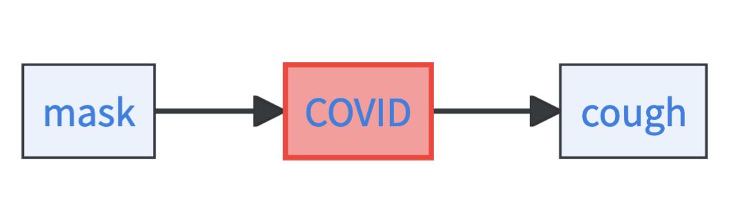
Let’s check out this simplified causal graph with only three variables: mask, COVID risk, and cough. Mask is causal for COVID risk and COVID is causal for cough. In this simple setting, you must specify three things to obtain a CBN:
- The marginal probability of wearing a mask, i.e. \(\mathbb{P}(\text{mask})\).
- The COVID risk for both people who either wear or don’t wear masks, that means \(\mathbb{P}(\text{COVID}\mid \text{mask}=0)\) and \(\mathbb{P}(\text{COVID}\mid \text{mask}=1)\).
- The probability of having a cough if the COVID risk is low or high, that means \(\mathbb{P}(\text{cough}\mid \text{COVID}=1)\) and \(\mathbb{P}(\text{cough}\mid \text{COVID}=0)\).
Let’s look at a toy example. Assume that 50% of people wear masks. Assume the COVID risk is 80% low / 20% high if people wear a mask and reversed if people do not wear a mask. And, the probability that people have a cough if they have a high COVID risk is 90%, and conversely, 10% if they have a low COVID risk.
Then, you can ask the following question and address it formally:
- Observational question: What is the probability of wearing a mask, having a high COVID risk, and not coughing? This can be computed by:
\[\begin{align*} &\mathbb{P}(\text{mask}=1, \text{COVID}=1, \text{cough}=0) \\ &=\mathbb{P}(\text{mask}=1) \times \mathbb{P}(\text{COVID}=1 \mid \text{mask}=1) \\ & \quad \times \mathbb{P}(\text{cough}=0 \mid \text{COVID}=1) \\ &= 0.5 \times 0.2 \times 0.1 = 0.01 \end{align*}\]
So this is a pretty unlikely combination. You can also ask a causal question, like:
- Interventional question: What is the probability of having a high COVID risk and cough if the policymaker enforces masks? This can be computed by:
\[\begin{align*} &\mathbb{P}(\text{COVID}=1, \text{cough}=1 \mid do(\text{mask}=1)) \\ &= \mathbb{P}(\text{COVID}=1 \mid \text{mask}=1) \times \mathbb{P}(\text{cough}=1 \mid \text{COVID}=1) \\ &= 0.2 \times 0.9 = 0.18 \end{align*}\]
Let’s generalize the ideas of this example. What do you need for a BCN?
- The marginal distribution \(\mathbb{P}(X_r)\) of all nodes in the causal graph without incoming arrows. These nodes are called root nodes.
- For all non-root nodes, you need their conditional distribution \(\mathbb{P}(X_j\mid pa_j)\) given their direct causes. The direct causes of a node are called parents.
If you have those two ingredients specified, you have a BCN. It allows you to compute both observational and interventional probabilities:
Observational probabilities:
\[\mathbb{P}(X)=\prod\limits_{i=1}^p \mathbb{P}(X_i | pa_i)\]
Interventional probabilities:
\[\mathbb{P}(X_{-j}\mid do(X_j=z))=\prod\limits_{\substack{i\neq j, \\j\not\in pa_i}}\mathbb{P}(X_i\mid pa_i) \prod\limits_{j\in pa_i}\mathbb{P}(X_i\mid pa_i,X_j=z)\]
To calculate interventional probabilities, you set the intervened variable to the desired value wherever it appears in the formula and the corresponding probability that the variable has this value to \(1\).
All of this is nice theory and toy modeling. But how about the real world where you do not magically have the BCN? Indeed, in practice, you can learn the BCN if you know the causal graph. All that differs between a BCN and a causal graph are marginal and conditional probabilities. If you have data, this is exactly where machine learning can help – estimating conditional probabilities. We generally advise estimating conditional probabilities with non-parametric machine learning models like neural networks or random forests, however, for small data sizes classical parametric approaches like maximum likelihood estimation or expectation maximization might be preferable [26].
10.6.2 Structural causal models allow you to reason about counterfactuals
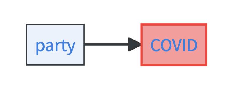
Interventional questions are often important if we want to act. But what if you want to explain why something has happened? Let’s say you got COVID and want to know why. Was it not wearing a mask? Or, was it that party last week? Or did you catch it in the metro from this guy who was sneezing heavily?
Answering why questions is always the most difficult, but usually also the most interesting. What is needed to answer such questions? You have to think through counterfactual scenarios. You know that you went to the party and you also know that you got COVID. To answer the why question, you need to find out how you got infected. Would you have got COVID if you hadn’t gone to the party? Would you have caught COVID if you hadn’t spoken to your charming but coughing neighbor at the party?
BCNs are not expressive enough to reason about counterfactual scenarios. Why not? Firstly, BCNs describe causal relations probabilistically on the level of groups of individuals who share certain features. Like the probability of getting COVID if everyone is forced to the party. The causal relationships are learned from data of people who did and of people who did not attend the party. The why question is more specific. It asks why you individually got COVID. Did you get COVID because you attended the party?4 Secondly, the fact that you got COVID is informative about you, it might reveal information about your properties on which there is no data. Like info about your immune system and how resilient it is against COVID. This information should not be ignored.
To answer why questions you need to simulate alternative scenarios, i.e. to perform counterfactual reasoning. A Structural Causal Model (SCM) is a model designed to simulate such alternative scenarios. Instead of describing probabilistic relationships in the data, a SCM explicitly models the mechanism that generates the data.
Let’s look at a super simple SCM with just two factors: whether you go to the party or not and whether you have COVID or not. These factors that you have explicit information about are called the endogenous variables.
The model moreover contains two exogenous variables. Exogenous variables describe background factors on which you have no data but which play a role in determining the endogenous variables. For example, whether you go to the party or not might be determined by whether you are in the mood for partying. Similarly, whether you get COVID or not might be influenced by how well your immune system is currently working. The exogenous variables are very powerful in SCMs. These factors completely determine the endogenous variables.
The SCM is thus specified by:
- Two noise terms: \(U_{\text{mood}}=Ber(0.5)\) describes whether you are in the mood for partying and the chances are fifty-fifty. \(U_{\text{immune}}=Ber(0.8)\) describes whether your immune system is up and the chances are pretty high (80%) that your immune system works well.
- One structural equation for the endogenous party variable, i.e. \(\text{party}:= U_{\text{mood}}\). Whether you go to the party is fully determined by whether you are in the mood for it.
- One structural equation for the endogenous COVID variable, i.e. \(\text{COVID}:=max(0,\text{party}-U_{\text{immune}})\). That means, you only get COVID if you are at the party and your immune system is down.
This SCM allows you to answer the counterfactual question: You went to the party and you caught COVID, would you have gotten COVID if you hadn’t gone to the party? Such counterfactuals are computed in three steps:
- Abduction: What does the fact that you got COVID tell you about the noise variables? Well, you could not have caught COVID with your immune system up. Thus, you can infer that \(U_{\text{immune}}=0\). Similarly, you know that you were in the mood for partying because otherwise, you would not have gone, i.e. \(U_{\text{mood}}=1\).
- Action: Let’s say you would not have gone to the party, that means you intervene and turn the party variable from one to zero, i.e. \(do(\text{party}=0)\).
- Prediction: What happens with the COVID variable if you switch party to zero? According to the structural equation of COVID, you only get COVID if both happens, you go to the party and your immune system is down. Thus, you do not get COVID.
In consequence, if you hadn’t gone to the party, you would not have caught COVID. So, you got COVID because you went to the party.
What if the counterfactual had not been true? Would partying still be a cause? Well, then things get more complicated. It could for instance be that you would have gone for sports instead of the party and caught COVID there. But partying would still have been the actual cause of you catching COVID. Search for actual causation to learn more about the topic.
Let’s generalize the ideas of the example. For a SCM, you need:
- A set of exogenous variables \(U\) that are determined by factors outside the model and independent from each other.
- A set of endogenous variables \(X\) that are fully determined by the factors inside the model.
- A set of structural equations \(F\) that describe for each endogenous variable \(X_j\) how it is determined by its parents and its exogenous variable \(X_j=f(pa_j, U_j)\).
Obtaining SCMs in real life is difficult. You may use machine learning to learn the structural equations if you know the causal dependencies between variables. However, even for that, you need quite some data, and making parametric assumptions can be advisable.
Like counterfactuals themselves, SCMs are highly speculative objects. There is no easy way to verify that a given SCM is correct, it always relies on counterfactual assumptions. Still, since humans reason in terms of counterfactuals all the time and are deeply concerned with why questions, it is nice to have a formalism that can capture counterfactual reasoning.
10.7 Learning causal graphs from data
Machine learning has revived an old idea – with enough data, we might be able to completely automatize science. In Part 1 and Part 2 of this chapter, you always needed a human scientist in the background. Someone to come up with interesting hypotheses, run experiments, or provide us with a causal graph. This part will be the most ambitious, it asks:
Can you get a causal graph just from data, without entering domain knowledge? This problem is often referred to as causal structure learning or causal discovery.
Didn’t we tell you in the beginning that observational data alone doesn’t do the trick? Correct! But it is intriguing to see how far you can go, especially if you add some additional assumptions. Clear the stage for a truly fascinating branch of research!
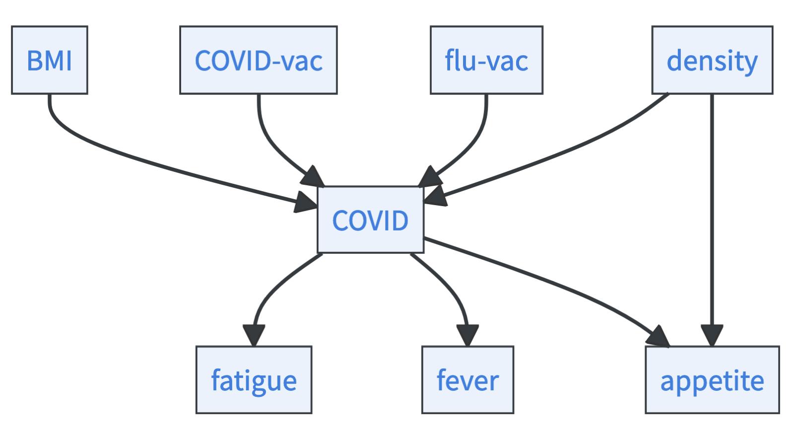
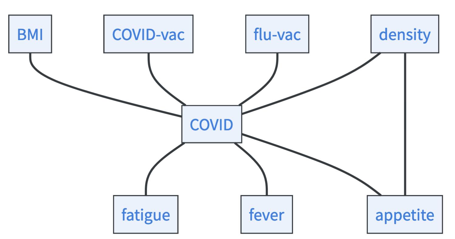
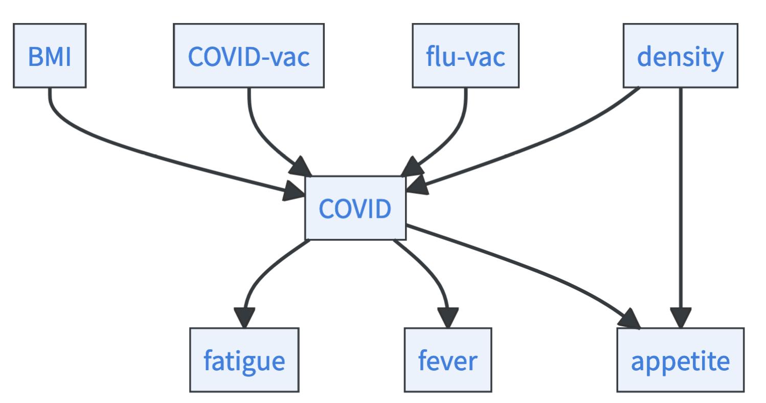
Imagine all you have is a dataset containing 5,000 entries. Each entry contains information about a person’s BMI, COVID vaccination status, flu vaccination status, COVID risk, fatigue, fever, appetite, and the density of population in the area the person lives in (Example based on [28] and [29]). The task is to structure these features in a causal graph – the problem of causal discovery. Let’s say the true graph that you want to learn looks like this:
Before you can approach this problem, you have to get some more background on how causal mechanisms, associations, and data relate to each other. The causal mechanism generates data. Within this data, features are associated with each other. That means that causal dependencies induce statistical (in-)dependencies. Particularly, if you have a causal graph, the so-called causal Markov condition applies:
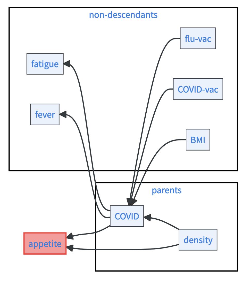
Given its parents in the causal graph, a variable is statistically independent of all its non-descendants. Or formally, let \(G\) be a causal graph and \(X_i\) be any variable in the network, then for all its non-descending variables \(nd_i\) holds \(X_i\perp \!\!\! \perp nd_i\mid pa_i\). Descendants of a given variable \(X_i\) are all the variables that can be reached from \(X_i\) by walking along the direction of arrows.
To get an intuition on the causal Markov condition, take a look at the graph below. Consider the variable appetite as an example. Its parents are COVID and density. Its nondescendants are BMI, COVID-vac, flu-vac, fever, and fatigue.5 The causal Markov condition allows you for example to say that appetite is statistically independent of fever if you know COVID and density. The formal way to write this is \(\;\text{appetite} \perp \!\!\! \perp \text{fever}\mid \text{COVID}, \text{density}\), where \(\perp \!\!\! \perp\) is the symbol for independence.
Cool, causal graphs induce statistical independencies, but what to do with that? Well, you have a dataset, so you can test for statistical independencies.
There are many different approaches to test such (conditional) independencies, and they vary regarding the parametric assumptions they pose. Some test the statistical dependency to be Gaussian or linear (e.g. partial correlation), or are tailored for categorical data like the chi-squared test [30]. Others allow for a greater variety of dependencies, like tests based on the Hilbert-Schmidt independence criterion (HSIC) [31]. The current trend goes even more non-parametric towards machine learning based tests for conditional independence. Questions of independence are translated into classification problems, where powerful machine learning models can be utilized (e.g. neural nets or random forests) [32], [33]. However, the fewer parametric assumptions you pose, the more statistical dependencies are possible. Thus, non-parametric tests usually have a very bad statistical power, which means you need a lot of data to identify independencies [34]. This problem gets worse the more variables you condition on – conditioning can be viewed as reducing the data you can test with. Incorrect conditional dependencies can lead to incorrect causal conclusions.
Let’s say you found a set of statistical independencies, how does this help you to learn the causal graph? Well, statistical independencies in the data are only compatible with certain kinds of causal structures. The data narrows down the causal stories that make sense. So the question is, how many faithful causal graphs (see the box: “Central assumptions in causality”) are compatible with the data?
As an example, assume you had only three variables: fatigue, COVID, and fever. By running statistical tests, you find that
- fatigue is independent of fever given COVID (Formally, \(\text{fatigue}\perp \!\!\! \perp \text{fever}\mid \text{COVID}\))
- None of the three variables is unconditionally independent of the other.
Then, three causal stories (causal chains) would explain this data.
- Story 1: \(\text{fatigue}\rightarrow \text{COVID}\rightarrow \text{fever}\).
- Story 2: \(\text{fatigue}\leftarrow \text{COVID}\leftarrow \text{fever}\).
- Story 3: \(\text{fatigue}\leftarrow \text{COVID}\rightarrow \text{fever}\) (called fork structure)
All of these stories (or causal graphs) are faithful and compatible with the given statistical (in-)dependencies. Also, one can show that there is no other causal graph that satisfies this.
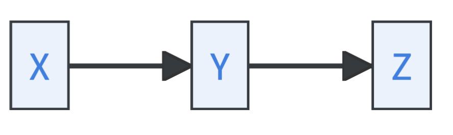
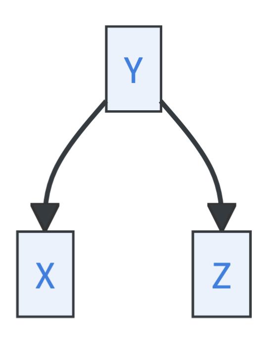
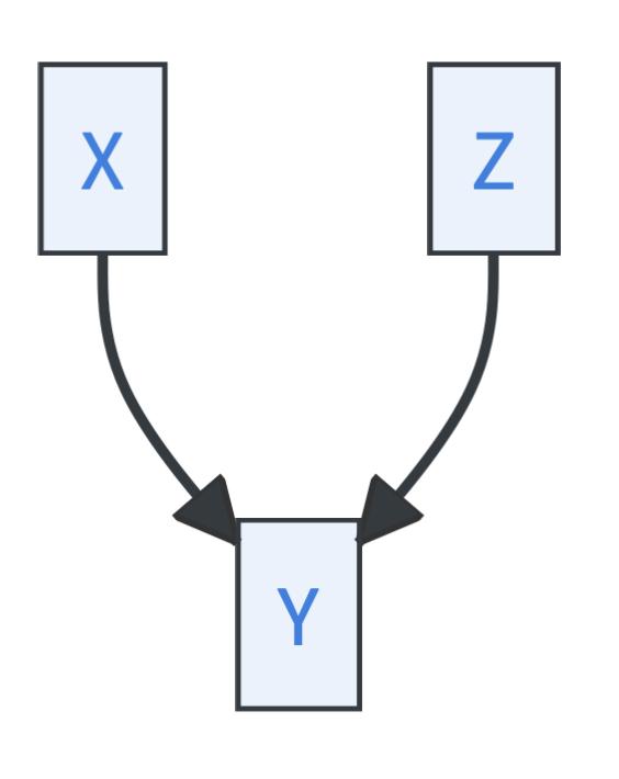
Let’s assume you have the variables \(X, Y\), and \(Z\). Three basic path structures in causal graphs are distinguished in causal discovery:
- Causal chains, where \(Y\) is called a mediator:
- Forks, where \(Y\) is called a common cause:
- Immoralities, where \(Y\) is called a collider:
Causal chains and forks imply identical conditional dependencies:
- \(X \perp \!\!\! \perp Z \mid Y\) (X and Z are independent given Y)
- X and Y are dependent
- X and Z are dependent
- Y and Z are dependent
Immoralities, however, exhibit a distinct pattern:
- \(X \perp \!\!\! \perp Z\) (X and Z are marginally independent)
- X and Z are dependent conditional on Y
- X and Y are dependent
- Y and Z are dependent
We call the set of faithful causal models that satisfies the same set of statistical (in-)dependencies the Markov equivalence class. How can you find the Markov equivalence class if all you have is a dataset? We provide one of many answers here, the so-called PC algorithm.6
The Peter-Clark (PC) algorithm: The most well-known algorithmic approach for finding the Markov equivalence class of causal models that is compatible with the statistical (in-)dependencies found in a dataset [36]. It requires causal sufficiency and the faithfulness condition to be satisfied. It runs the following steps:
Identify the skeleton: We start with a fully connected network with undirected arrows. Then, step by step we look through all unconditional and conditional independencies between features. We start with unconditional independencies, continue with independencies conditional on one variable, then two, and so on. If two features are (conditionally) independent, we erase the arrows between them. In the end, we get the so-called skeleton graph without directed arrows.
- Unconditional independence: By running a statistical test, we learn that BMI, COVID-vac, flu-vac, and density are all pairwise independent. This allows us to erase the arrows between those variables.
- Independence conditioned on one variable: Conditioning on COVID makes fatigue, fever, and appetite pairwise independent. Moreover, BMI, COVID-vac, flu-vac, and density become independent of fatigue and fever. We can erase all arrows between these variables.
- Independence conditioned on two variables: If we condition on COVID and density, BMI, COVID-vac, and flu-vac become independent of appetite. We can therefore erase all arrows between appetite and these variables.
- We find no further independencies. So this is our resulting skeleton!
Identify immoralities: Immoralities are paths of the form \(X\rightarrow Y\leftarrow Z\) that lead to unique (in)dependencies, namely to \(X\perp \!\!\! \perp Z\) and \(X,Z\) are dependent conditional on \(Y\). We can use this uniqueness to orient some arrows. Go through all unconditional independencies \(X\perp \!\!\! \perp Z\) where the nodes are connected via one intermediate variable \(Y\), check whether conditioning on \(Y\) makes them dependent. If yes, you found an immorality and can orient the arrows.
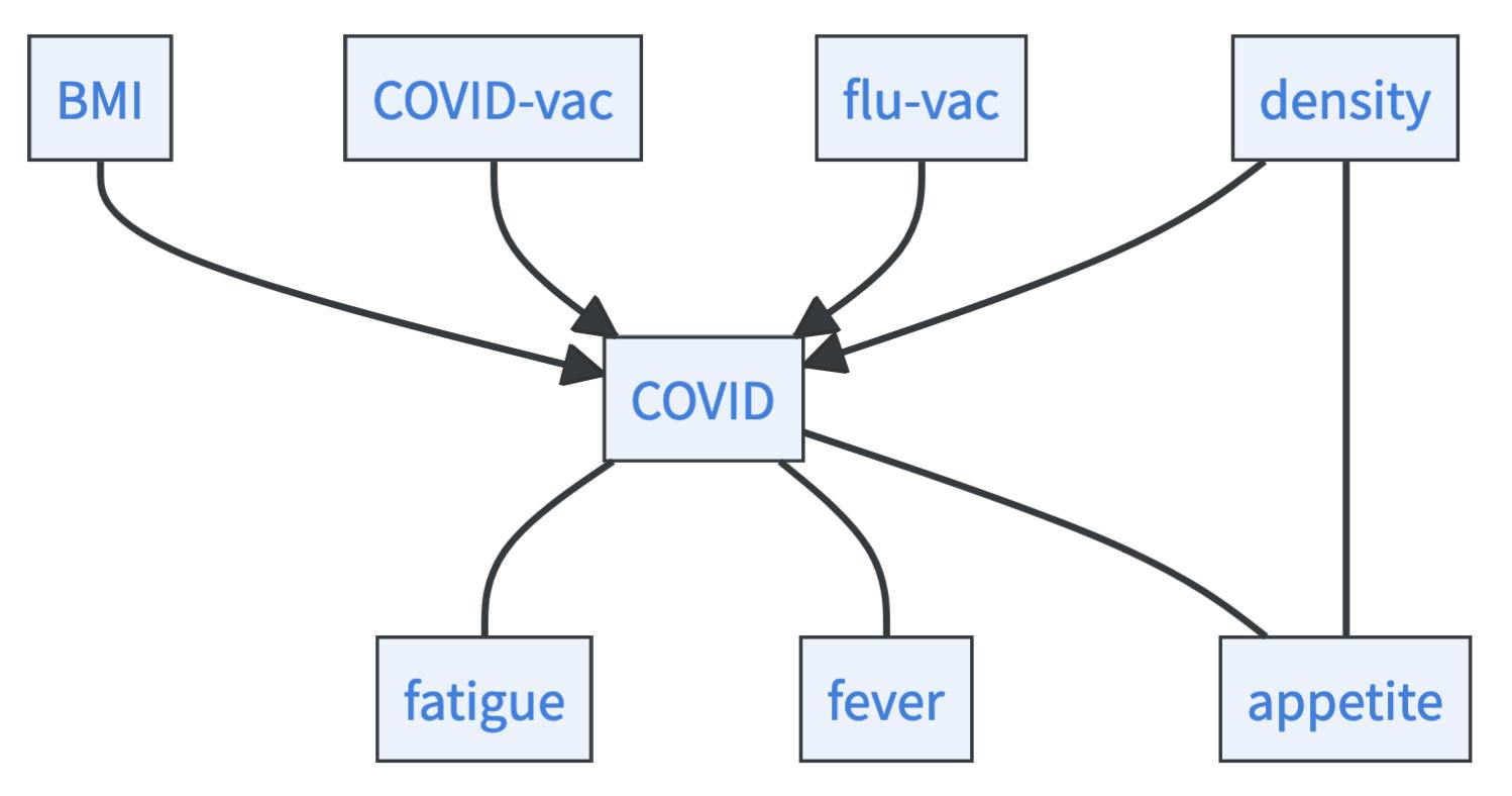
- As you can see, in our skeleton all arrows are undirected. We now check for all unconditionally independent variables that become dependent if we condition on one variable. This is the case for BMI, COVID-vac, flu-vac, and density. They are unconditionally independent but become dependent if we condition the COVID variable. We can therefore orient some arrows in our graph.
Apply logic: Now you have identified all immoralities. Thus, if you find three variables that are connected like this \(X\rightarrow Y-Z\) where the arrow between \(Y\) and \(Z\) is undirected, you can infer that \(X \rightarrow Y \rightarrow Z\), because otherwise there would be another immorality that you must have discovered. Also, we search for an acyclic graph. So if there is only one way to avoid making a cycle, that is the way you orient the arrows.
- Which arrows would lead to new immoralities? If fatigue, fever, and appetite had arrows towards COVID, new immoralities would emerge that would have been found in the statistical testing. Thus, they must have arrows coming from the COVID variable. Now only one arrow is left undirected, the arrow between density and appetite. If this arrow would go from density towards appetite, there would be a cycle: \(\text{COVID}\rightarrow \text{appetite}\rightarrow \text{density}\rightarrow \text{COVID}\). Thus, the arrow must go from density to appetite.
Cool, we were able to identify the full causal graph just from the (in-)dependencies! But we were lucky. If we had looked at a more complex graph, the PC algorithm would have spit out a graph where some arrows are left unoriented. All possible ways for orienting these remaining arrows define the Markov equivalence class. But can you go further? Is there a way to identify the correct causal model among the Markov equivalence class? You need something extra for this:
- Perform real-world experiments: You could simply run experiments. There are proven bounds for how many experiments you have to perform to identify the correct causal graph. For instance, if multi-node interventions are allowed, \(log_2[n]+1\) interventions are sufficient to identify the causal graph, where \(n\) is the number of nodes [37].
- Pose more assumptions: One of the most prominent assumptions for the identifiability of the causal graph is the linearity of the relationship and non-Gaussian noise terms in the structural equations. Alternatively, you can assume non-linearity and the additivity of noise. Check out [30] to learn more. Most approaches rely on the idea that the noise variables are independent in one but not in the other causal direction.
You can see causal models as devices for interpreting data. But when are the interpretations correct? Only if certain assumptions are satisfied. Causality is therefore a deeply assumption-driven field. The most crucial ones are listed here:
- Causal sufficiency: This is one of the key assumptions in the field. It is sometimes also referenced as the assumption of no unobserved confounders. It means that you have not missed a causally relevant variable in your model that would be a cause of two or more variables in the model. This assumption is not testable and without it, far less can be derived [38].
- Independence of mechanisms: Means that causal models are modular. Intervening on one structural equation does not affect other structural equations. Or on a probabilistic take, changing the marginal distribution of one variable does not affect the conditional distributions where this variable acts as a causal parent. This assumption seems almost definitional to mechanistic modeling and implies the independence of the exogenous noise terms [30].
- Faithfulness: Is connected to how to interpret causal graphs probabilistically. Faithfulness means that every causal dependence in the graph results in a statistical dependence. Note that it is hard to justify faithfulness in finite data regimes [39].
- Positivity: For every group of the population, you have both subgroups with and without treatment. This is crucial when it comes to treatment effect estimation. If positivity is violated, you extrapolate (non-)treatment effects for certain subgroups, which can go terribly wrong.
This list is far from complete, there are many more, such as consistency, exchangeability, and no interference [16], [40]. The correctness of your interpretations of data with causal models or the causal models you may partially derive from data are extremely sensitive to these assumptions. If possible, check if they apply!
10.8 Learning causal representations from data
Causal discovery only makes sense if the features are meaningful representations and you can talk meaningfully about their causal relationships. This is the case with highly structured, tabular data that has been heavily pre-processed by the human mind. But the data you often have, especially the data you want to analyze with machine learning, doesn’t look like that, it consists of:
- images made of pixels
- texts made of letters
- sounds made of frequencies
For example, it makes no sense to construct a causal model where the variables are single pixels. However, it may be meaningful to talk about the causal relationships between objects in images. How can you go from pixels to these objects? How can you get meaningful higher-order representations from lower-order features?7
Machine learning is a field concerned with learning higher-order representations. Causal representation learning therefore describes a dream that many in machine learning share – the dream of fusing symbolic approaches like causal models with modern machine learning. This would combine the strengths of both worlds: learning complex meaningful representations from data AND reasoning symbolically in a transparent and logical manner.
Indeed, doing so is extremely difficult and the research in this field is still in its infancy. Machine learning models learn complex representations to perform their predictions, however, whether the representations are in any sense similar to the ones humans form or at all understandable to us is an open question. Adding labels to the representations you want and modifying the loss function to use these representations might be one way to go [42]. But it is data costly! Is there a way to make sure that machine learning models learn meaningful representations that could be used to construct causal models? Can you maybe even build in constraints informed by your understanding of causality to learn such representations? We’ll give you some hunch in this direction…
Autoencoders consist of two parts. An encoder maps the input to a higher-order representation and a decoder maps the higher-order representation back to the original input space. The only difference in a variational autoencoder is that input is encoded into a set of parameters of a probability distribution, whereas the decoder takes a sample from this distribution and maps it back to the original input space. VAEs are (unlike the rest of the book) unsupervised learning techniques. They allow, among other things, to compress high-dimensional information into low-dimensional features with little or no loss of information.
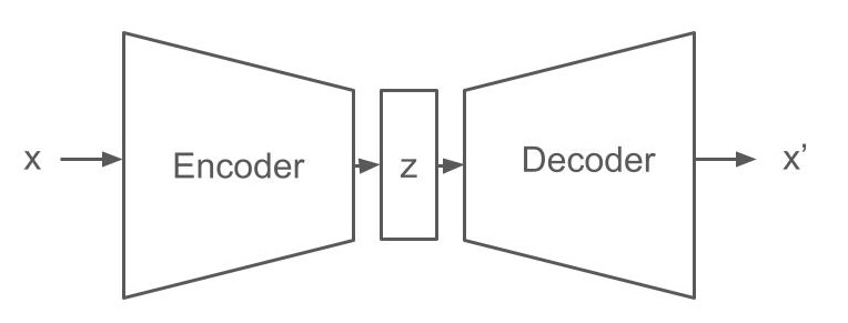
Putting causal constraints in variational autoencoders: You can see the probability distributions in the middle of VAEs as abstractions of the low-level features your data lives in. Therefore, VAEs are constantly discussed in the context of representation learning in general and there are many ways to incorporate knowledge about these representations both via the architecture and the loss function [43]. Instead of learning representations and then looking at how you can incorporate them in causal models, you can do the reverse and ask: What makes representations good candidates for causal models and how can such knowledge be incorporated into the VAE framework? Since research on the topic is still in its infancy, we will only provide a list of a few ideas inspired by [44] :
- Sparsity: One key idea in causality is that a few powerful representations are enough to explain all kinds of complex phenomena. This can for example be enforced by the size of the middle VAE layer.
- Generality across domains: Powerful representations are useful across tasks. What makes them useful is that they capture robust patterns in nature. You can enforce this for instance in VAEs by training them to use the same representations for different decoding tasks.
- Independence: First, if two representations contain the same information, one of them is redundant. But you want to have simple models to efficiently communicate about the world. Second, the core idea in causality is that you have independent sources of variation and that you can disentangle these sources and their interactions. One approach for achieving this in VAEs is modifying the loss to make sure that the representations in the intermediate layer are statistically independent.
- Human interventions: What makes a variable suitable for causal modeling is that you can intervene upon it. Thus, 42 % of randomly selected atoms from a table do not constitute a good representation, as you cannot use or intervene in these 42% in isolation. This human-centered causal bias can be entered into VAEs for example through video data, where objects are constantly moved and intervened upon but stay persistent.
- Simple relationships: Causal models are rarely densely connected. Instead, a handful of causal relationships between higher-order variables give rise to the associations you observe in the world. This inductive bias of simplicity can be enforced via the decoder architecture or the loss function.
10.9 Causality helps to formulate problems
After finishing this chapter, you may feel a little overwhelmed. A lot of theoretical concepts were presented and at the same time, there was little practical advice, e.g. compared to the domain-knowledge chapter (see Chapter 8). We have the impression that the link between causal theory and the practical problems of scientists is underdeveloped in current research. For example, there are only a few examples where causal discovery algorithms have been used to gain insights from practice.
Nevertheless, we believe that every researcher should be familiar with the concepts presented above, such as the Reichenbach principle, treatment effect estimation, and causal modeling. Causality is what many of you are ultimately looking for when you want to control, explain, and reason about a phenomenon. While causality as a field does often not provide ready-made practical solutions, it offers you a language to formulate your problem and describe possible solutions.
Many of the chapters in this book are closely related to causality:
- Some domain knowledge (see Chapter 8) you want to encode may be causal.
- Many questions addressed via model interpretation (see Chapter 9), such as algorithmic recourse, are ultimately causal questions [29].
- Causality is one leading approach to improving robustness (see Chapter 11) [45].
- Approaches for better uncertainty quantification, such as conformal prediction (see Chapter 12) are currently being integrated into causal inference [46].
There is also an association between COVID risk and the FIFA football ranking [4]. Here, the causal story is spuriously Messi…↩︎
Saitama is the protagonist of the anime series “One-Punch Man” who defeats his opponents with just one punch. In one of the episodes, he accidentally damages good old Jupiter.↩︎
There are two general approaches for estimating treatment effects with machine learning, model-agnostic and model-specific techniques. Model-specific techniques are based on a certain class of machine learning models, such as GANITE for neural nets [18] or causal forests for random forests [19]. Model-specific techniques often come with the advantage of valid confidence intervals. Other techniques are model agnostic, which means, you can simply plug in any machine learning model into the estimation. The T-Learner and Double Machine Learning we present here are examples of such model-agnostic approaches. Today, there are tons of approaches to estimating causal effects with machine learning, check out [20] or [21] to learn more.↩︎
In the literature, it is differentiated between counterfactuals and actual causes [27].↩︎
The parents are indeed also non-descendants. However, the conditional independence you can derive from the causal Markov condition between \(E\) of \(C\) given you know \(C\) holds trivially for an arbitrary variable by \(\mathbb{P}(E,C\mid C)=\mathbb{P}(E,C,C)/\mathbb{P}(C)=\mathbb{P}(E\mid C)=\mathbb{P}(E\mid C)\mathbb{P}(C\mid C).\)↩︎
The PC algorithm is already quite old but great for understanding the general idea of causal discovery. There are many extensions, generalizations, and alternatives of PCs on the market. We point you to [30] for an overview and to [35] for an R package implementing standard causal discovery algorithms.↩︎
Causal abstraction is a cool framework for thinking about the relationship between low-level and high-level causal representations [41]. Science is all about causal models at different levels of description, think of the relationship between physical models, chemical models, and biological models.↩︎