9 Interpretability
What’s your biggest concern about using machine learning for science? A survey [1] asked 1600 scientists this question. “Leads to more reliance on pattern recognition without understanding” was the top concern, which is well-founded: Supervised machine learning is foremost about prediction, not understanding (see Chapter 2).
To solve that problem, interpretable machine learning was invented. Interpretable machine learning (or explainable AI1) offers a wide range of solutions to tackle the lack of understanding. Interpretability, in the widest sense, is about making the model understandable to humans [4]. There are plenty of tools for this task, ranging from using decision rules to applying game theory (Shapley values) and analyzing neurons in a neural network. But before we talk solutions let’s talk about the problem first. Interpretability isn’t a goal in itself. Interpretability is a tool that helps you achieve your actual goals. Goals that a prediction-focused approach alone can’t satisfy.
The integration of domain knowledge eliminated many childhood diseases of machine learning. The Ravens began building larger and larger models to study increasingly complex phenomena. Krarah approached Rattle with a question: “The models must have learned so many interesting relationships, is there any way to extract this knowledge?” Rattle nodded and winked at Krarah. Recently, Raven Krähstof wrote a book about interpretable machine learning.

9.1 Goals of interpretation
Imagine you model the yield of almond orchards. The prediction model predicts almond yield in a given year based on precipitation, fertilizer use, prior yield, and so on. You are satisfied with the predictive performance, but you have this nagging feeling of incompleteness that no benchmark can fill. And when you find a task can’t be solved by performance alone, you might need interpretability [5]. For example, you might be interested in the effect of fertilizer on almond yield.
We roughly distinguish three interpretability goals (inspired by [6]):
- Discover: The model may have learned something interesting about the studied phenomenon. In science, we can further distinguish between confirmatory (aka inference) and exploratory types of discovery. In the case of almond yield, the goal might be to study the effect of fertilizer.
- Improve: Interpretation of a model can help debug and improve the model. This can lead to better performance and higher robustness (see also Chapter 11). Studying feature importance you might find out that the prior yield variable is suspiciously important and detect that a coding error introduced a data leakage.
- Justify: Interpretation helps to justify a prediction, or also the model itself. Justification ranges from justifying a prediction towards an end-user touching upon ethics and fairness, to more formal model audits, but also building trust through, e.g. showing coherence with physics. For example, you are trying to convince an agency to adapt your model, but first, you have to convince them that your model aligns with common agricultural knowledge.
The goals interact with each other in the life cycle of a machine learning project. For example, to discover knowledge, your model should show good performance. However, building a performative model is an iterative process in which interpretability can immensely help by monitoring the importance of features.
But how do you achieve interpretability for complex machine learning models? To oversimplify, the field of interpretable machine learning knows two paths: interpretability-by-design and post-hoc interpretability. Interpretability-by-design is about only using interpretable, aka simple models. Post-hoc interpretation is the attempt to interpret potentially complex models after they were trained.
9.2 Interpretability-by-design
Interpretability by design is the status quo in many research fields. For example, quantitative medical research often relies on classical statistical models, with logistic regression being a commonly used model. These statistical models are considered inherently interpretable because they often relate the features to the outcome through a linearly weighted sum in one way or another. Statistical models are also dominant in the social sciences and many other fields. The use of a linear regression model to predict almond yield is not unheard of [7]. However, models with very different motivations can also be interpretable by design, such as differential equations and physics-based simulations in fields such as physics, meteorology, and ecology.
If you value interpretability, you might decide that you only use machine learning algorithms that produce interpretable models. You would still approach the modeling task in a typical performance-first manner, but restrict our solutions to be only models that you deem interpretable. It would still be about optimization, but you strongly limit the hypothesis space, which is the pool of models that are deemed okay to be learned.
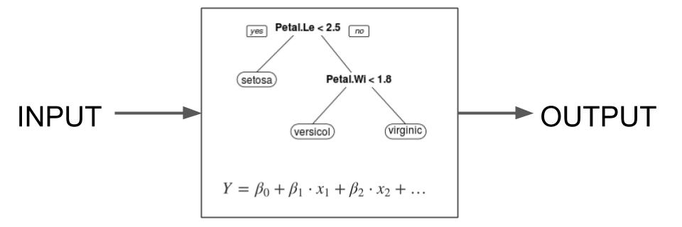
Interpretable machine learning models may include:
- Anything with linearity. Essentially the entire pantheon of frequentist models. Linear regression, logistic regression, frameworks such as generalized linear models (GLMs) and generalized additive models (GAMs), …
- Decision trees. Structures that present the prediction in the form of typical but not necessarily binary trees that are split by features.
- Decision rule lists
- Combinations of linear models and decision rules such as RuleFit [8] and model-based trees [9]
- Case-based reasoning
Researchers continue to invent new machine-learning approaches that produce models that are interpretable by design [10], but there’s also controversy as to what even constitutes an interpretable model [11]. Arguably, not even a linear regression model is interpretable if you have many features. Others argue that whether a particular model can be seen as interpretable depends on the audience and the context. But whatever your definition of interpretation: By restricting the functional form of the models, it becomes functionally better controllable. Even if you can argue that linear regression isn’t as easy to interpret, then it is still true that the model contains no interactions (at least on the input space of the model). And models that are interpretable by design, or at least structurally simpler, can help with goals such as discovery, improvement, and justification.
- Discover: A logistic regression model allows insights about the features that increase the probability of, e.g., diabetes.
- Improve: Regression coefficients with a wrong direction may signal that a feature was wrongly coded.
- Justify: A domain expert can manually check decision rules.
Interpretability by design has a cost: Restricting the hypothesis may exclude many good models and you might end up with a model that is worse in performance. The winners in machine learning competitions are usually complex gradient-boosted trees (e.g. LightGBM, catboost, xgboost) for tabular data and neural networks (CNN, transformer) for image and text data. It is not the models that are interpretable by design that are cashing in the price money.
Besides lower performance, interpretability-by-design has a conceptual problem when it comes to discovery (inference). To extend the interpretation of the model to the real world, you have to establish a connection between your model and the world. In classical statistical modeling, for example, you make lots of assumptions about what the data-generating process might be. What’s the distribution of the target given the features? What’s the process of missing values? What correlation structures do you have to account for? Other approaches such as physics-based simulations also have a link between the model and the world: it is assumed that certain parts of the simulation represent parts of the world. For interpretability by design, there is no such link. For example, there is no justification for saying that almond yield is produced by decision tree-like processes.
Another problem is performance: What do you do when you find models that have better predictive performance than your interpretable one? A model that represents the world well should also be able to predict it well. You would have to argue why your interpretable model better represents the world, even though it predicts it less well. You might have just been oversimplifying the world for your convenience. This weakens any claims to link the model to reality. An even worse conceptual problem is the Rashomon effect [12].
Rashomon is a 1950 Japanese film. It tells the story of a murdered samurai from four different perspectives: a bandit, the samurai’s wife, the samurai’s spirit communicating through a psychic, and a commoner observing the event. While each perspective is coherent in itself, it is incompatible with the other three stories. This so-called Rashomon effect has become an established concept in law, philosophy, and, as you can see, statistics and machine learning.
The Rashomon effect describes the phenomenon that multiple models may have roughly the same performance, but are structurally different. A head-scratcher for interpretation: If optimization leads to a set of equally performant models with different internal structures, then you can’t pick one over the other based purely based on an argument of performance. An example: Decision trees are inherently interpretable (at least if short) but also inherently unstable – small changes in the data may lead to very different trees even if the performance might not suffer too much. If you use a decision tree for discovery, then the Rashomon effect makes it difficult to argue that this is the exact tree that you should even be interpreting.
The verdict: Inherently interpretable models are much easier to justify than their more complex counterparts. However, using them for insights (inference) has conceptual problems. Fortunately, there’s also the class of post-hoc interpretation methods, for which we have a theory of how their interpretation may be extended to the modeled phenomenon.
9.3 Model-specific post-hoc interpretability
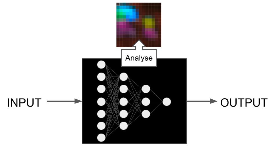
Instead of opposing model complexity, you can also embrace it and try to extract insights from the complex models. These interpretability methods are called post-hoc, which translates to “after the event”, the event being model training. Post-hoc methods can be either model-specific or model-agnostic: Model-specific interpretation methods work with the structure of the model, whereas model-agnostic methods treat the model as a black box and only work with the input-output data pairs. Model-specific methods are tied to a specific model type and require that you inspect the model, for example:
- Gini importance leverages the splitting criterion in decision trees to assign importance values to features
- Transformers, a popular neural network architecture, has an attention layer that decides which part of the (processed) input to attend to for the prediction. Attention visualization is a model-specific post-hoc approach to interpret transformers.
- Activation maximization approaches assign semantic meaning to individual neurons and layers: What concept maximally activates each neuron?
- Gradient-based explanation methods like Grad-CAM or layer-wise relevance propagation (LRP) make use of neural network gradients to highlight the inputs that affected the predictions strongly
Model-specific methods occupy an odd spot in the interpretability space. The underlying models are usually more complex than the interpretability-by-design ones and the interpretations can only address subsets of the model. For most interpretation goals, model-specific post-hoc interpretation is worse than interpretability-by-design.
When it comes to inference, model-specific methods share the same conceptual problem with interpretability by design: If you want to interpret the model in place of the real world, you need a theory that connects your model with the world and allows a transfer of interpretation. Model-specific approaches, as the name says, rely on the specific model they are building, and such a link between model and reality would require making assumptions about why this model’s structure is representative of the world, which are probably invalid [13]. However, they still may be useful in pointing out associations for forming causal hypotheses (see Chapter 10).
The line is blurred between interpretability by design and model-specific post-hoc interpretation. You might see a linear regression model as inherently interpretable because the coefficients are directly interpretable as feature effects. But what if you log-transform the target? Then you also have to transform the coefficients for interpretation. You can argue that this is still interpretable by design, but you can add many modifications that make the model stray further from interpretability heaven. And for interpretation, you rely more and more on post-hoc computations, like transforming the coefficients, visualizing splines, etc.
Now that we are done talking down on model-specific interpretation, let’s talk about our favorite methods: model-agnostic interpretation techniques. And yes, we make no secret out of this, but we are quite the fans of model-agnostic interpretation.
9.4 Model-agnostic post-hoc interpretation methods
You are tasked to write a manual for the world’s weirdest vending machine. Nobody knows how it works. You tried to open it but decided against inspection for fear of breaking the machine. But you have an idea of how you could write that manual. You start pressing some of the buttons and levers until, finally, the machine drops an item: a pack of chips with the flavor “Anchovies”. Fortunately, they are past the due date. You feel no remorse throwing them away. The other good news is that you made the first step toward writing that manual. The secret: Just try things out systematically and find out what happens.
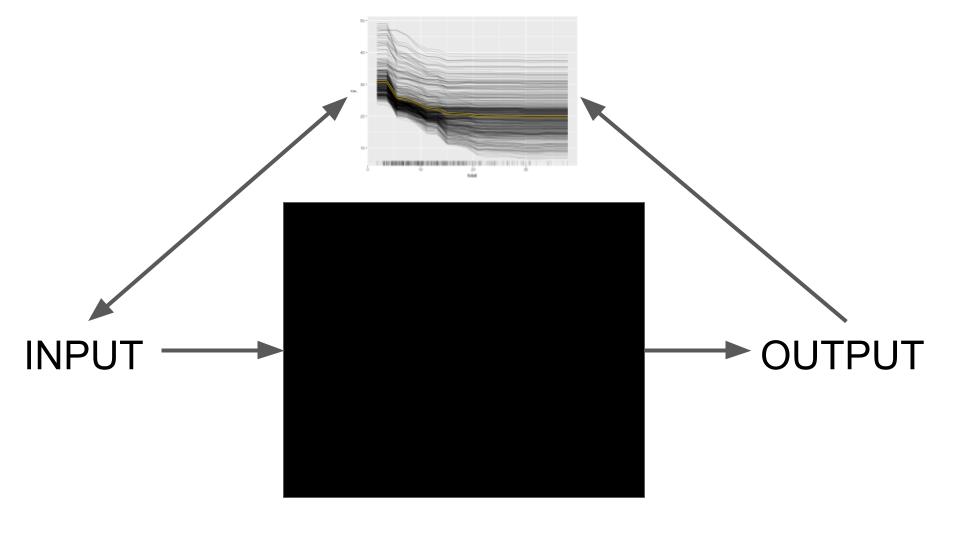
The fictive almond yield model is just like the vending machine. By intervening in the input features, the output (aka the prediction) changes and you can gather information about the model behavior. The recipe is to sample data, intervene in the data, predict, and aggregate the results [14]. And that’s why model-agnostic interpretation methods are post-hoc – they don’t require you to access the model internals or change the model training process. Model-agnostic interpretation methods have many advantages:
- You can use the same model-agnostic interpretation method for different models and compare the results.
- You are free to include pre- and post-processing steps in the interpretation. For example, when the model uses principal components as inputs (dimensionality reduction), you can still produce the interpretations based on the original features.
- You can apply model-agnostic methods also to inherently interpretable models like using feature importance on decision trees.
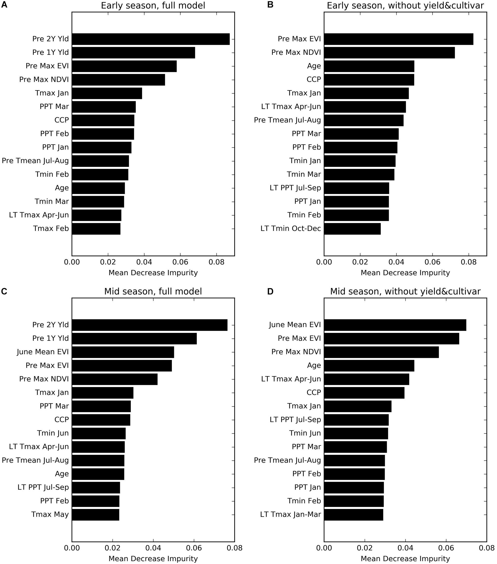
One of the simplest model-agnostic to explain is permutation feature importance: Imagine the almond yield researcher wants to know which features were most important for a prediction. First, they measure the performance of the model. Then they take one of the features, say the amount of fertilizer used, and shuffle it, which destroys the relationship between the fertilizer feature and the actual yield outcome. If the model relies on the fertilizer feature, the predictions will change for this manipulated dataset. For these predictions, the researchers again measure the performance. Usually, shuffling makes the performance worse. The larger the drop in performance, the more important the feature. Figure 9.1 shows an example of permutation feature importance from the almond yield paper [15].
PFI is one of many model-agnostic explanation methods. This chapter won’t introduce all of them, because that’s already its own book called Interpretable Machine Learning [16] and you can read it for free! But still, we’ll provide a brief overview of the interpretability landscape of model-agnostic methods. The biggest differentiator is local versus global methods:
- Local methods explain individual predictions
- Global methods interpret the average model behavior.
9.4.1 Local: Explaining individual predictions
The almond researchers might want to explain the yield prediction for a particular field and year. Why did the model make this particular prediction? Explaining individual predictions is one of the holy grails of interpretability. Tons of methods are available. Explanations of predictions attribute, in one way or another, the prediction to the individual features.
Here are some examples of local model-agnostic interpretation methods:
- Local surrogate models (LIME) [17] explain predictions by approximating the complex model locally with a neighborhood-based interpretable model.
- Scoped rules (anchors) [18] describe which feature values “anchor” a prediction, meaning that within this range, the prediction can’t be changed beyond a chosen threshold.
- Counterfactual explanations [19] explain a prediction by examining which features to change to achieve a desired counterfactual prediction.
- Shapley values [20] and SHAP [21] are attribution methods that assign the prediction to individual features based on game theory.
- Individual conditional expectation curves [22] describe how changing individual features changes the prediction.
9.4.2 Global: Interpreting average model behavior
While local explanations are about data points, global explanations are about datasets: they describe how the model behaves, on average, for a given dataset, and, by extension, the distribution that the dataset represents.
We can further separate global interpretability:
- Feature importance methods [23] rank features by how much they influence the predictions. Examples:
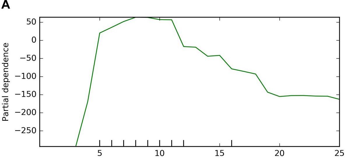
- Feature effect methods describe how features influence the prediction. We can further divide feature effect methods into main and interaction effects: Main feature effects describe how an isolated feature changes the prediction, as shown in Figure 9.2. Interaction effects describe how features interact with each other to influence the predictions. Examples:
We see global interpretation methods as central, especially for discovery.
9.4.3 Interpretation for scientific discovery
How useful is model-agnostic interpretation for scientific insights? Let’s start with two observations:
- Interpretation is first and foremost about the model.
- If you want to extend the model interpretation to the world, you need a theoretical link.
Let’s say you model the almond yield with a linear regression model. The coefficients of the linear equation tell you how the features linearly affect the yield. Without further assumption, this interpretation concerns only the model. In classical statistical modeling, a statistician might make the assumption that the conditional distribution of yield given the features is Gaussian, that the errors are homoscedastic, that the data are representative, and so on, and only then carefully make a statement about the real world. Such results in turn may have real-world consequences, such as deciding the fertilizer usage.
In machine learning, you don’t make these assumptions about the data-generating process but let predictive performance guide modeling decisions. But can we establish a theoretical link between the model interpretation and the world maybe differently? We’ve discussed that establishing this link isn’t easy when it comes to model-specific interpretation:
- You would have to justify whether the specific model structures represent the phenomenon you study. That’s unreasonable for most model classes: What reason do you have to believe that phenomena in the world are structured like a decision rule list or a transformer model?
- The Rashomon effect presents you with an unresolvable conflict: If different models have similar predictive performance, how can you justify that the structure of one model represents the world, but the others don’t?
But there’s a way to link model and reality via model-agnostic interpretation. With model-agnostic interpretation, you don’t have to link model components to variables of reality. Instead, you interpret the model’s behavior and link these interpretations to the phenomenon [27]. This, of course, also doesn’t come for free.
- You have to assume there is a true function \(f\) that describes the relation between the underlying features and the prediction target (see Section 12.5.2 for theoretical background on this true function).
- The model needs to be a good representation of function \(f\) or at least you should be able to quantify uncertainties.
Let’s make it more concrete: The almond researcher has visualized a partial dependence plot that shows how fertilizer use influences the predicted yield. Now they want to extend the interpretation of this effect curve to the real world. First, they assume that there is some true \(f\) that their model \(\hat{f}\) tries to approximate, a standard assumption in statistical learning theory [28].
The partial dependence plot is defined as:
\[PDP(x) = \mathbb{E}[\hat{f}(x_j, X_{-j})]\]
and estimated with:
\[\frac{1}{n} \sum_{i=1}^n \hat{f}(x_j, x_{-j}^{(i)})\]
The index indicates the feature of interest, and \(-j\) indicates all the other features. You can’t estimate the true PDP because \(f\) is unknown, but you can define a theoretical partial dependence plot on the true function by replacing the model \(\hat{f}\) for the real \(f\): \(PDP_{true}(x) = \mathbb{E}[f(x_j, X_{-j})]\).
That allows you, at least in theory and simulation, to compare true PDP with estimated PDP, as visualized in Figure 9.3.
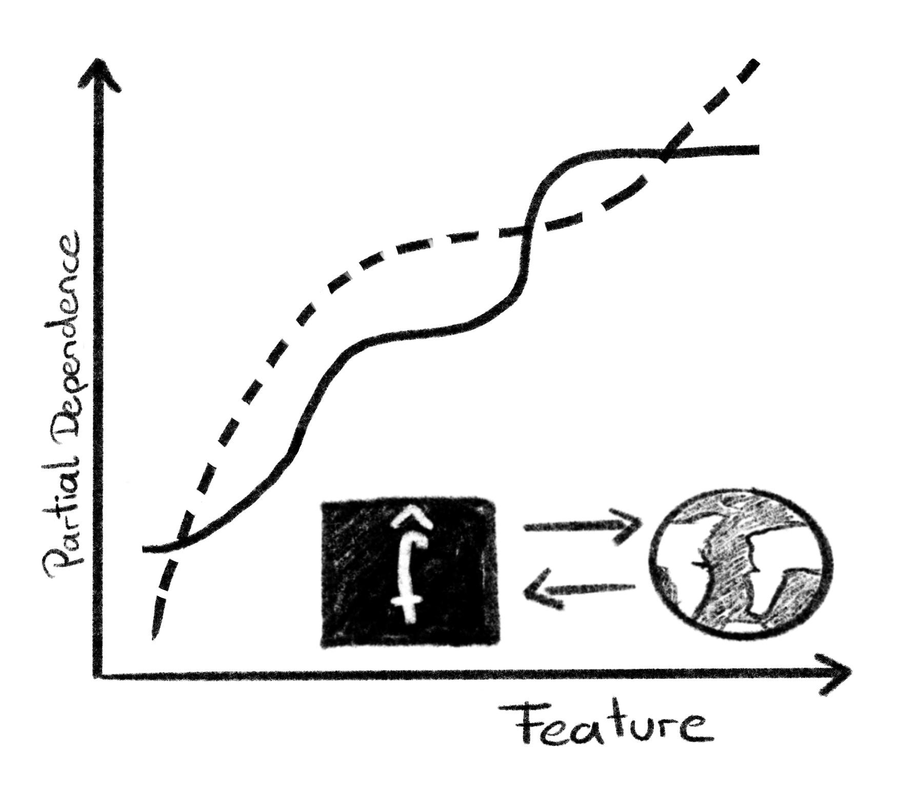
That’s what we have done in [29] and discussed more philosophically in [27].2 We’ll give an abbreviated sketch of our ideas here. The error between the true and the model PDP consists of 3 parts:
- The model bias describes the bias of your learning algorithm.
- The model variance describes the algorithm’s variance over datasets from the same distribution.
- The estimation error describes the variance that arises from estimating the PDP empirically.
Ideally, you can either reduce or remove each source of uncertainty or at least quantify them. The model bias is the toughest part: You can’t easily quantify it because it would require you to know the true function \(f\). A way to reduce the bias is to train and tune the models well and then assume that the model’s bias is negligible, which is a strong assumption to make, of course. Especially considering that many machine learning algorithms rely on regularization which may introduce a bias to reduce variance. An example of model bias: If you use a linear model to model non-linear data, then the PDP will be biased since it can only model a linear relation.
The model variance is a source of uncertainty that stems from the model itself being a random variable since the model is a function of the training data, which is merely a sample of the distribution. If you would sample a different dataset from the same distribution then the trained model might come out slightly different. If you retrain the model multiple times with different data (but from the same distribution), you get an idea of the model’s variance. This makes model variance at least quantifiable.
The third uncertainty source is the estimation error: The PDP, like other interpretation methods, is estimated with data, so it is subject to variance. The estimation error is the simplest to quantify since the PDP at a given position \(x\) is an average for which you know the variance.
In our paper, we showed that permutation feature importance also has these 3 sources of uncertainty when comparing model PFI with the “true” PFI. We have conceptually generalized this approach to arbitrary interpretation methods in [27]. While we haven’t tested the approach for all interpretation methods in practice, our intuition says it should be similar to PDP and PFI. This line of research is rather new and we have to see where it leads. To justify using machine learning + post-hoc interpretation as an inference about the real world this alone might be too thin. But then again, many researchers already use machine learning for insights, so having some theoretical justification is great to have.
There’s one challenge to interpretability that gives us bad dreams, specifically for the goal of insights: correlated features.
9.5 Correlation may destroy interpretability
When features correlate with each other, model-agnostic interpretation may run into issues. To understand why, let’s revisit how most model-agnostic methods work: Sample data, intervene in the data, get model predictions, and aggregate the results. During the intervention steps, new data points are created, often treating features as independent.
For example, to compute the permutation importance of the feature “absolute humidity” for the almond yield model, the feature gets shuffled (permuted) independently of the other features such as temperature. This can result in unrealistic data points of high humidity but low temperatures. These unrealistic new data points are fed into the model and the predictions are used to interpret the model. This may produce misleading interpretations:
- The model is probed with data points from regions of the feature space where the model doesn’t work well (because it was never trained with data from this region) or even makes extreme predictions.
- Unrealistic data points shouldn’t be used for the interpretation, as they aren’t representative of the studied reality.
- Features don’t independently change in the real world
Given these issues, why do many still use so-called “marginal” methods for interpretation that treat features as independent? Two reasons: 1) It is technically much easier to, for example, shuffle a feature independently compared to shuffling the feature in a way that preserves the correlation. 2) In an ideal world, you want a disentangled interpretation where you can study each feature in isolation.
In practice, you can avoid or at least reduce the problem of correlated features with these approaches:
- Study correlations between features. If they are low, you can proceed with the usual marginal version of the interpretation methods.
- Interpret feature groups instead of individual features. For most interpretation methods you can also compute the importance or effect for an entire group of features. For example, you can compute the combined PFI for humidity and precipitation by shuffling them together.
- Use conditional versions of the interpretation methods. For example, conditional feature importance [30], conditional SHAP [31], M-Plot and ALE [26] and subgroup-wise PDP and PFI [32], Leave-one-covariate out (LOCO) [33].
The third option, conditional interpretation, is more than a technical fix.
Let’s say you want to shuffle the humidity feature to get its importance for almond yield. It is correlated with temperature, so you have to ensure that new data points respect the correlation structure. Instead of shuffling humidity independently, you sample it based on the values of temperature. The first data point has a high absolute humidity, you draw the temperature feature based on this high humidity. This leads to the “permuted” humidity feature to respect the correlation with precipitation, while breaking the relation with the yield target.
Conditional intervention changes the interpretation. For example, for permutation feature importance, the interpretation changes to: Given that the model has access to temperature, how important is it to know the humidity in addition? The more complex the dependence structures between features are, the more complex the (conditional) interpretation becomes. To use conditional interpretation, you must understand how the interpretation changes compared to the marginal versions. But on the other side, we’d argue that conditional interpretation is the way to go, especially for the goal of insights. Not only because it fixes the extrapolation problem, but also because for insights you are interested in how the features are related to the target regardless of the model.
9.6 Interpretability is just one part
Model interpretability alone might not solve your problems. Rather, it is strongly interlinked with the other topics covered in this book.
- Interpretability for scientific insights is tightly linked to generalization (see Chapter 7). If you aren’t aware of how the data were collected and which population the dataset represents, it is unclear what to do with the conclusions from model interpretation.
- When you justify the model for your boss, your colleague, or your peers, it is by showing the model coheres with domain knowledge (see Chapter 8).
- Understanding causality (see Chapter 10) is crucial for interpretation. For example, a feature effect may be rather misleading if confounders are missing from the model.
What do interpretability and explainability exactly mean? Even researchers in this field can’t decide on a definition [2]. From an application-oriented perspective, it is most useful to treat these terms interchangeably. Under these keywords, you find approaches that allow you to extract information from the model about how it makes predictions. We use the definition from [3]: Interpretability is about mapping an abstract concept from the models to an understandable form. Explainability is a stronger term that requires interpretability and additional context.↩︎
Our work on extending interpretation for insights is what motivated us to write the book you are reading.↩︎