11 Robustness
Machine learning systems should not only work under laboratory conditions – they should work in the wild! And yes, we mean that in the true sense of the word.
Imagine you are an animal ecologist studying the diversity and conservation of species in the Serengeti. You know that machine learning systems allow you to identify, count, and even describe animals from images alone, as illustrated in Figure 11.1. There are tons of motion sensor cameras throughout the Serengeti. Together with the predictions by the machine learning model of Norouzzadeh et al. [1], you’ll soon have an amazing dataset to tackle your research questions.
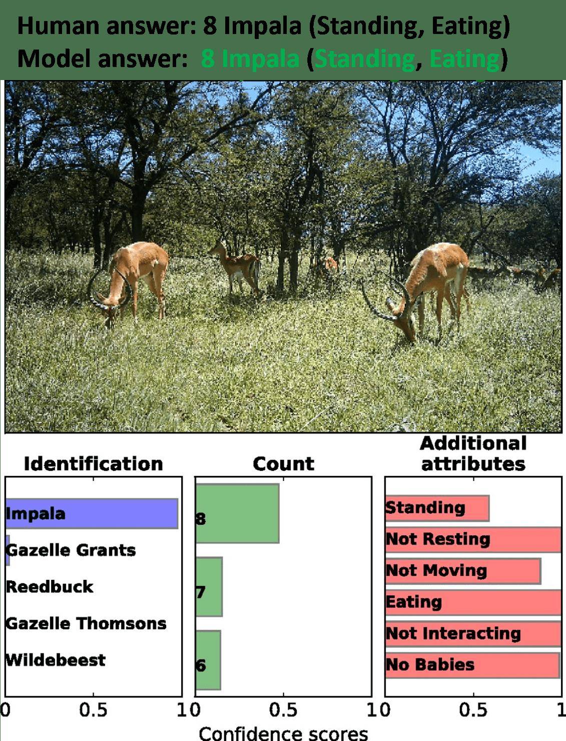
Norouzzadeh et al. [1] have indeed done an impressive job with their machine learning model: Their ensemble of trained convolutional neural networks (CNN) achieves 94.9% accuracy on the Snapshot Serengeti dataset [2] – that is a comparable performance to human labelers. Sounds like a reliable tool to build your research on, right?
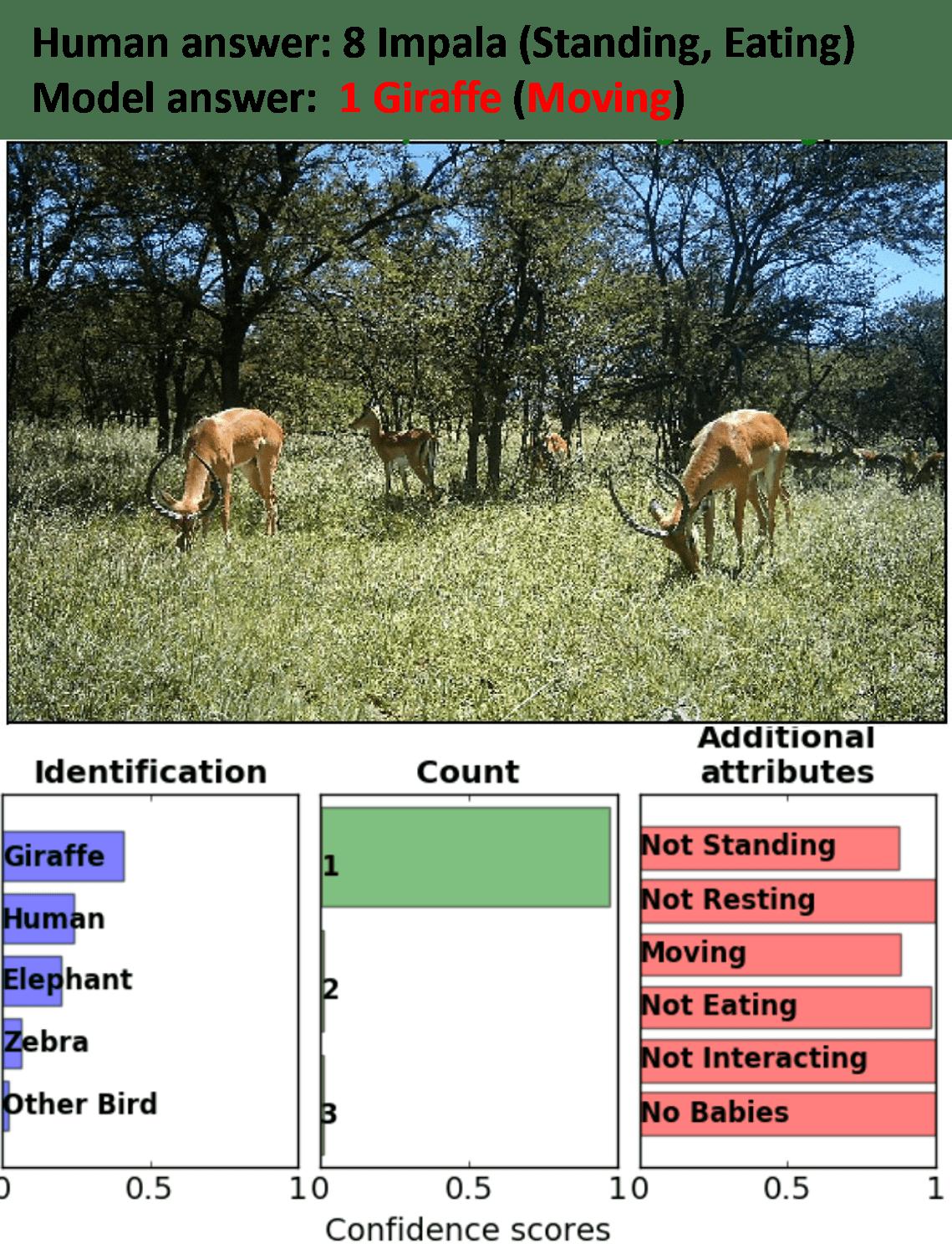
To human eyes, Figure 11.2 is the same image as Figure 11.1, but for the model, it is not. The model gets it all wrong now: the species, the count, and even the description. What has happened? The image is a so-called adversarial example. All current machine learning models, especially image classifiers, are susceptible to such well-engineered variations in the input that are imperceptible to the human eye but lead the prediction model astray. But Norouzzadeh et al. [1] didn’t do anything wrong. Quite the contrary! The paper is a role model for machine learning in science:
- They explain in detail how they deal with class imbalances in the data and target leaks (see Chapter 7), which can occur because the camera sensors take three photos in succession.
- They take into account label noise and conduct confidence thresholding (see Chapter 12).
- They report overall performance and class performance (see Chapter 14) and provide usable open-source code (see Chapter 13).
Still, what should we make of the fact that machine learning models are not robust to adversarial examples?
Adversarial examples have kicked off the robustness debate in machine learning [3], and we will explore their occurrence in some detail at the end of this chapter Section 11.7. But not any image would fool the animal classifier, the model performs quite well on real images taken in the wild.
We believe that scientists should not get sleepless nights from deceiving artificial input data that never occurs in practice. In science, there is usually no adversary that deceives your model – except perhaps Reviewer 2. As you will see in this chapter, there are many more profound robustness issues in machine learning that should worry you!
Machine learning not only found its way into science, but its products became global bestsellers. Krarah’s former Ph.D. students wanted to get their piece of the pie and turn the tornado prediction idea into a startup. But there was a problem. While the original model worked perfectly in their home territory, it was useless in other countries. They asked Rattle for a workshop to teach them about robust machine learning.

11.1 What does robustness mean?
In everyday language, robustness is a property of a single entity. A washing machine can be robust if it works for many years without trouble. A person can be robust if she can handle many situations competently. However, this leaves open what robustness is really about except for functioning well in general.
To detect robustness problems and solve them systematically, you need a language that allows you to operationalize robustness [4]:
- Robustness target is the thing that should be robust. For example, you may be interested in how robust the performance of the animal classifier is.
- Robustness modifier is the thing with respect to which the robustness target should be robust. For example, this could be the images on which you apply your animal classifier.
- Modifier domain specifies the relevant changes in the modifier to which the target should be robust. For example, this could be changes in the background lighting of the images.
- Target tolerance specifies how much the target is allowed to change if the modifier changes within the modifier domain. For example, you might be fine if the model performance decreases a bit for images with a darker background as long as the performance does not drop drastically.
So what does robustness mean?
Definition: A robustness target is robust with respect to a modifier if relevant interventions to the modifier within the domain do not lead to greater changes than specified by the target tolerance.
We can now talk in a more nuanced way about robustness. For example, the wildlife image classifier performance (robustness target) is relatively robust to changes in the lighting conditions when taking the images (relevant interventions). However, it is less robust to targeted modifications (irrelevant interventions) on the input pixels. Ultimately, to judge whether your model is suitable for a specific application, you have to check if it is robust to relevant interventions on modifiers. This forces you to think about the changes you expect to occur in deployment!
11.2 Auditing and robustifying strategies
Broadly speaking, robustness researchers have to adopt two different perspectives:
- Auditing: Is your model performance robust to relevant modifier changes? For example, you can check how the animal classifier performs when you darken the background of the test data.
- Robustifying strategies: What can you change in data collection and model selection to make your model more robust to relevant modifier changes? For example, if you train your model with more images taken at night, your model will generally perform better in this environment.
Both aspects are interacting. You may audit the model and detect potential robustness weaknesses. To mitigate these weaknesses, you apply robustifying strategies. But what should you audit for?
11.3 Understand data distribution shifts
In practice, the most crucial modifier is the data. Your training data may stem from one source, but when you now deploy your model, the data may look entirely different. There are different sources of data distribution shifts:
- Natural shifts occur because the natural conditions change. If you think of the animal classifier, you have to deal with:
- varying weather or lighting conditions,
- changes in the flora and fauna over time, or
- new camera sensors placed at novel locations.
- Performative shifts are induced by the model itself and its effects on the data. Imagine a model that predicts which diseases a person will develop based on their behavior. Provided with these predictions, the person may change her behavior and thus invalidate the prediction.
- Adversarial shifts occur due to attackers who modify the data. An example is given in Figure 11.2.
For natural scientists, the most important distribution shifts are natural distribution shifts, whereas social scientists must care just as much about performative shifts. Adversarial shifts are more of a problem in business or industry applications but less so in science.
You can also distinguish different types of data distribution shifts. Data in supervised machine learning is described as pairs \((x^{(i)}, y^{(i)})_{i=1, \ldots, n}\) sampled from an underlying distribution \(\mathbb{P}(X,Y)\), where \(X:=(X_1,\dots,X_p)\) describes the input features and \(Y\) the target variable. We can express the different types of data distribution shifts directly through the distributions of \(X\) and \(Y\):
- Covariate shift describes a case where the distribution \(\mathbb{P}(X)\) has changed. In the example above, a covariate shift can occur if a camera was previously in the open sun but is now in the shade of a plant.
- Label shift describes a case where the distribution \(\mathbb{P}(Y)\) has changed. The installation of a new camera in the previously ignored riverine forests in the Serengeti, for example, will lead to many more hippos being observed.
- Concept shift describes a case where the conditional distribution \(\mathbb{P}(Y\mid X)\) has changed. In the example of wildlife, this can happen when there is a new categorization of species; previously there is only the gazelle category, but afterward it is subdivided into Grant’s gazelle, Thomson’s gazelle, and so on.
Again, understanding what type of distribution shift you face can be vital for robustifying your model. But before we come to robustifying strategies, let’s first look into robustness audits.
11.4 Strategies to audit for robustness
Has the distribution shift already occurred? Or are you only anticipating a distribution shift? This determines which audit you can perform:
- Post-hoc audit: The distribution shift has occurred already. You have collected new data after the shift and can evaluate the quality of your model on this data. In the wildlife example, you may have only trained your model with data from the dry season, and now, in the middle of the wet season, you want to evaluate the model’s performance.
- Anticipatory audit: The distribution shift has not yet occurred. So you have no data about the expected changes. For example, if you are in the dry season and want to predict how your model will work in the wet season.
11.4.1 Post-hoc audit
A post-hoc audit is comparably simple – just analyze your model performance on your data. For example, you might want to compare the model performance between dry (pre-shift) and wet season data (post-shift).1
Understand whether and how the data differs
But how can you even recognize that the distribution has shifted? You need to constantly monitor your data and check the data properties. For tabular data, there are a variety of summary statistics like the mean values, standard deviations, ranges, or correlation coefficients. The situation is similar for text, where you have word frequencies, word lengths, similarity of word embeddings, cosine similarity, or text sentiment. When these statistics start to vary, your distribution shift alarm bells should ring. For image data, we lack good summary statistics. Instead, eyeballing data samples through time taking into account domain knowledge can be more effective.
There are also modality-independent automated strategies for detecting data distribution shifts – called out-of-distribution (OOD) detection [5]. We discuss them below in Section 11.5.2.
Analyze the different errors
Just as important as understanding the distribution shift itself is understanding how it affects model performance. Comparing performance before and after the shift is only the tip of the iceberg of a proper audit. False positive or false negative rates may also differ, and you could have contextual preferences for either bounding false positives or false negatives. Similarly, we recommend to group and compare errors across output classes.
Interpretation methods can point to the sources of errors
Interpretation methods (see Chapter 9) give you insight into the features on which the model relies upon and how these features impact model performance. Feature attribution techniques, for example, allow you to analyze the attention of image classifiers for specific predictions. You should be alerted if the model classifies Grant Gazelles by looking at the background rather than the animals [6]. If you deal with tabular data, you may compare global feature importances based on data before against after the distribution shift.
11.4.2 Anticipatory audit
An anticipatory robustness audit is more demanding than a post-hoc audit. The shift has not occurred yet – so you have no data from after the shift. You need to specify the shift qualitatively based on the sources and types of shifts above. To also quantify the effect of an anticipated shift on model performance, you additionally have to generate synthetic data that reflects the shift.
Specify the shift qualitatively
What shift do you expect, a natural or a performative shift? Is it a shift in covariates, in labels, or even in concepts? Be careful to specify the shift correctly. For example, auditing your model for adversarial robustness in a non-adversarial setting is pointless. Consult your domain knowledge! What aspects of your domain do you expect to vary and to which of the above types of shifts do they belong? Think back to our wildlife example: researchers are aware that there are relevant seasonal effects on the Serengeti environment and its wild inhabitants.
Generate (semi-)synthetic data and systematically test your model on it
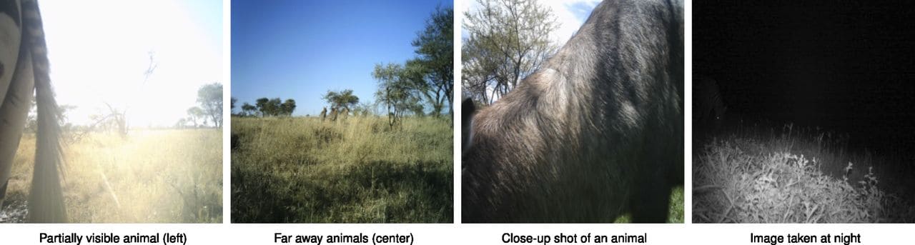
To perform a quantitative audit, you need data that reflects the distribution shift. But because you don’t observe but only anticipate the shift, you have to generate data synthetically. You have to translate your qualitative knowledge about the shift into a way to generate data. We discuss various strategies to generate data below in Section 11.5.3, for example, image filters allow you to turn day data into night data (see Figure 11.4).
Suppose you have created a synthetic dataset, does this mean you finally reached the point you start at in a post-hoc audit? Yes and no, there remain two big differences: 1. You already have a profound understanding of the data because you generated it. 2. The insights your synthetic data offer depend on your assumptions about the shift.
Interpretation methods allow you to anticipate shifts
Interpretation methods allow you to perform an audit without specifying the expected distribution shift or synthetic data. Instead, you simply analyze your pre-distribution shift data in a more explorative way, e.g. if feature attribution methods indicate that the model relies on background features like trees to classify an animal, this could mean that the model performs worse under varying background conditions. This alerts you to both the potentially dangerous distribution shift (changes in background) and the reason why your model is failing (reliance on background). Similarly, if a spurious feature has a large feature importance, your model may fail in settings where this feature varies; A COVID risk predictor trained in Munich that relies on street names is likely to fail in Paris. Finally, feature effect methods such as individual conditional effect curves (ICE) and counterfactual explanations describe model behavior in relevant counterfactual scenarios.
What you need to audit your model for, depends heavily on the application context. The wildlife model, which acts as a labeling tool, requires less extensive auditing than machine learning-based medical diagnosis. What audits are needed depends on the risks of errors, the instability of the environment, and other domain characteristics. For high-risk applications like in medicine, there are often additional legal requirements, such as those set out in European AI legislation and in medical device regulations.
11.5 Strategies to robustify your model
Say your audit has shown that your model is not robust to relevant distribution shifts. How can you robustify it? This is a list of common robustifying strategies, ordered by their position in the machine learning pipeline. Each of the strategies is discussed in more detail below:
- Control the source: Some shifts are under the control of the model authority. For example, the purchase of a new brand of camera sensor can lead to greater distribution shifts than sticking with the old brand.
- Filter out-of-distribution data: You could train a second model to filter out data that significantly differs from the training data. For example, the machine learning model should not provide predictions for animals that are not included in the training set, leaving these cases for human labelers.
- Gather data representative of the shift: You may gather additional (real or synthetic) data that accounts for the shift. For instance, one could use image filters to augment wet season data using dry season data.
- Carefully select and construct features: The lack of robustness in your model may be due to its reliance on incorrect features or improper feature encoding. For instance, by removing the image background, shifts in the background will no longer affect the model’s performance.
- Choose inductive biases wisely: Some shifts can be accounted for by adjusting your modeling assumptions (see Chapter 8). For counting animals, you may choose an architecture that generalizes to high animal counts like sequential subtizing [7].
- Transfer learning to obtain robust representations: Often, your model is sensitive to distribution shifts because its learned representations overfit the training data. In such cases, transfer learning – reusing representations learned by other models trained on the same data modality – can help. Norouzzadeh et al. [1] demonstrate that transferring representations from common image classifiers increases the data efficiency of the wildlife classifier.
The strategies you should choose to robustify your model should be informed by your audit. If you caused the distribution shift yourself, you might be able to control the shift. When your model performs poorly only on rare anomalies, filtering out these cases might be the best approach. If the distribution shift is unavoidable and causes a significant performance drop, the most common strategy is to augment your data and retrain the model. If the distribution shift is unavoidable but data augmentation is difficult, you may need to engineer features, adjust the modeling assumptions, or use transfer learning.
11.5.1 Control the source
It is usually not like distribution shifts are just happening and there is nothing you can do about them. You often have an active role – you caused the distribution shift by an action. You installed a camera sensor from a different brand and suddenly the performance drops? You put food next to the camera to spot more animals and suddenly your animal count bound reaches its limits? In some cases, rather than adapting the data or the model, it can be smarter to tackle the very source of the shift. You must enact control to guarantee a stable environment, e.g. by using only cameras from the same brand.
But not all distribution shifts are within your control. You cannot keep the Serengeti in the wet season all year. Other sources you can control but not without unwanted side effects: You can create stable lighting conditions around the camera, but this can attract or repel certain animals.
11.5.2 Filter out-of-distribution data
There will always be data that presents a challenge for your model. Especially data that is very different from the training data. Out-of-distribution (OOD) detectors enable you to filter out data on which your model would perform substantially worse. These data can then be handled separately, e.g. by a human labeler. Thereby, OOD detection robustifies overall performance in deployment. However, OOD detectors only act as filters; they do not help with substantial distribution shifts.
How to find out if a data point is OOD? With OOD detectors! Sometimes people further differentiate between methods designed to detect anomalies (rare data from different distributions), novelties (data from a shifting distribution), or outliers (rare data within training distribution) [5], [8]. Here, we focus on OOD detection more generally. There are four different approaches [5]:
- Classification-based methods phrase OOD detection as a classification problem. Some classification-based methods require data labeled as within and outside of the distribution. Others leverage uncertainty-aware classifiers and label data with high classification uncertainty as OOD.
- Density-based methods model explicitly the probability density of the training data. Data whose density lies below a certain threshold is labeled as OOD.
- Distance-based methods calculate the difference of a given data point to the centroid or prototypes in a dataset. Data whose distance surpasses a certain threshold is labeled OOD.
- Reconstruction-based methods use autoencoder methods to detect OOD data. Data with higher reconstruction error are labeled as OOD.
To get an overview of all the different types of OOD detectors check out the review papers by [8], [5], and [9].
Reconstruction-based techniques have advantages over the other approaches: Unlike classification-based methods, you do not need to label data as (non) OOD; Unlike density-based methods, you do not need to specify a model of the probability density; And unlike distance-based methods, you do not need to construct complex reference points such as centroids or prototypes. Let’s therefore take a deeper look into reconstruction-based OOD detectors.
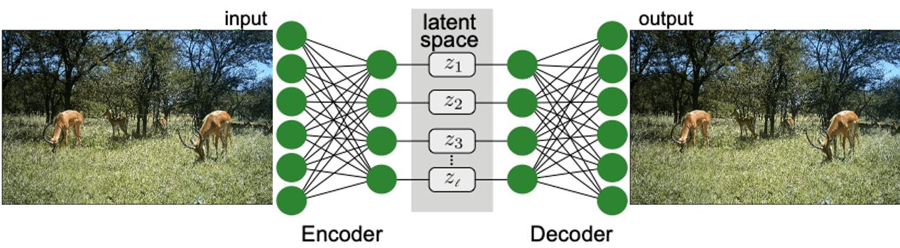
Autoencoders describe a neural-network-based method to project high-dimensional inputs into a low-dimensional feature space (often called latent space) with a minimal loss of information. This is achieved through a two-stage architecture:
- Encoder: Projects the high-dimensional input into a prespecified low-dimensional latent space.
- Decoder: Maps the projected inputs from the latent space back to the original space.
The encoder and decoder mappings are optimized to minimize the reconstruction error of the training data. The reconstruction error of a given input describes the difference (according to some metric) between this input and the output we obtain after sequentially encoding and decoding the input. In our example, this would mean calculating the mean squared error between the initial Impala image and its reconstructed version that runs through the encoder and decoder network.
Out-of-distribution detection with autoencoders
Say \(x\) is the data point you want to classify as within or outside of the training distribution. Then the encoder network can be described as a mapping \(E:\mathbb{R}^h\rightarrow \mathbb{R}^l\) from a high-dimensional feature space \(\mathbb{R}^h\) to a low dimensional latent space \(\mathbb{R}^l\). Similarly, the decoder network is a mapping \(D:\mathbb{R}^l\rightarrow \mathbb{R}^h\) and \(L\) is a distance function on the input space \(\mathbb{R}^h\) (e.g. mean squared error). Then, the reconstruction error of \(x\) is defined as: \[\text{RE}(x):=L(x,E(D(x))).\] This allows us to define a simple OOD detector: \[\text{OOD}(x):=\begin{cases} \text{OOD}\quad\quad \text{if RE}(x)>\tau \\ \text{not OOD}\quad \text{else} \end{cases}\] Intuitively, any data with a reconstruction error above a certain threshold \(\tau\) counts as OOD. This primitive approach faces clear limitations:
- Also OOD data can have low reconstruction error. By extending the reconstruction error with the Mahalanobis Distance on the latent space, this problem can be tackled [11].
- Training autoencoders is hard, you have to make architectural choices based on domain knowledge (e.g. CNN for images), define an appropriate latent space (i.e. just the right size to capture the training distribution without information loss), and choose an appropriate loss function [8].
- Training autoencoders requires representative training data [9], but in practice, the data is often unbalanced.
11.5.3 Gather data representative of the shift
Why are distribution shifts a problem for machine learning models? In the case of a covariate shift (i.e. shift of \(\mathbb{P}(X)\)) or a label shift (i.e. shift of \(\mathbb{P}(Y)\)), your model fails because it has never seen this kind of data and is unable to extrapolate. In the case of a concept shift (i.e. shift in \(\mathbb{P}(Y\mid X)\)), your model may have faced similar inputs but the learned dependencies became unreliable.
In any case, the most prominent solution in the research literature for how to robustify your model to such shifts is the same – gather more data that reflects the distribution shift! There are two strategies to obtain such data:
- Gather real labeled data with active learning: You may want real labeled data. Active learning concerns the systematic search for data worth labeling.
- Augment your data: Gathering real data comes with high costs and you have limited control over which kind of data you get. Data augmentation is concerned with generating synthetic instances using domain knowledge.
Active learning
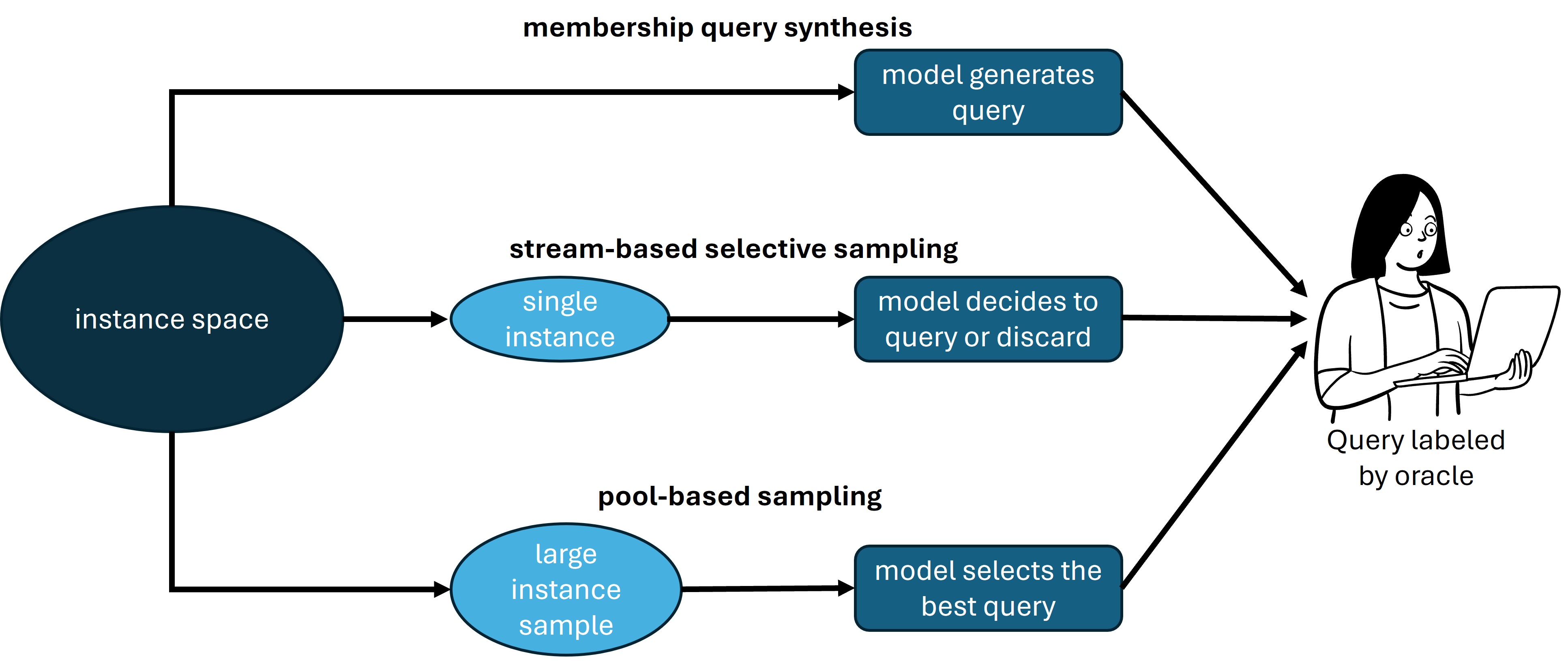
Which data should you label to robustify your model? Labeling all data is often too expensive and time-consuming. The literature differentiates three active learning setups, based on how the labeler receives the data [12]:
- In membership query synthesis any input in the input space is a potential candidate for labeling, even completely unrealistic inputs.
- In stream-based sampling you receive data sequentially and have to decide whether to label this data.
- In pool-based sampling you receive a big data sample and have to choose a subsample that you want to label.
Active learning is largely concerned with the automation of the selection process for labeling [12], [13]. The data selection process can be based on high prediction uncertainty, proximity to the decision boundary, randomness, expected model error, expected training effect, or data representativeness. In the example, Norouzzadeh et al. [1] suggest labeling those wildlife images with the highest prediction uncertainty. Note that all these different active learning strategies are readily available in recent Python packages like modAL [14] and ALiPy [15].
You may also have intuitions about what data to track and label. Incorporating such knowledge [16] and interacting with the model through interpretability techniques [17] can significantly improve active learning strategies.
Data augmentation
Data augmentation is about creating synthetic data. Wait, don’t you also need active learning to label these data? In some cases yes, namely if you want to find the label for an arbitrary input. However, when we talk about data augmentation, we usually create data for which we know the label. Data augmentation has been particularly the focus in computer vision [18], [19], but recently there is growing literature on data augmentation in the context of natural language processing [20].
There are two general strategies to augment your data [18]:
- Data transformation: Transformations applied to labeled data that are known not to change the label. Selecting the right transformations is an excellent way to incorporate domain knowledge. Focus on transformations you expect to occur in practice.
- Data synthesis: Creation of entirely new data with known labels. Data synthesis may be based on generative models or Computer Aided Design (CAD) models. The aim is to generate synthetic data that shares important properties with your training data but varies from it in relevant aspects.
In computer vision, there are geometric transformations (changing the angle, position, direction, or size of an image) and photometric transformations (changing attributes like coloring, saturation, contrast, or camera artifacts). Some transformations concern the overall image, while others only concern one region. Transformations may delete, replace, swap, or recombine regions of the image.
In natural language tasks, it is common to randomly insert, delete, or swap words in a sentence or to substitute words in sentences with their synonyms. If you have a trained language model, also more sophisticated transformations can be performed, such as: back translation, where sentences are translated back and forth between two languages; text paraphrasing, where the same content is rephrased without changing the meaning; and style transformations, where the same content is described in different styles (e.g. more formal vs less formal language).
Data synthesis is more challenging. Computer-aided design (CAD) allows you to model physical objects by hand and perform various geometric and photometric transformations in a physically adequate way. Neural rendering learns 3D scene representations from 2D images and thereby avoids hand-crafted CAD modeling. The most common approach to data synthesis in computer vision is using generative models like generative adversarial networks (GANs) or variational autoencoders (VAEs). The models generate realistic images that can be sampled conditionally on a desired target class. In natural language processing, the best generator models are large language models like ChatGPT or LLaMA, which can be prompted to generate data with a certain content.
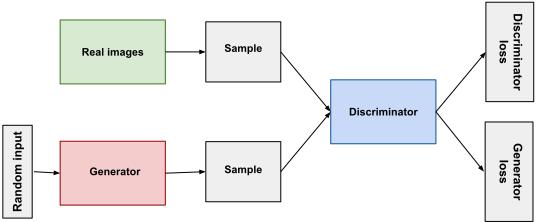
A GAN is a generative model that allows the generation of highly realistic data [21]. It is trained using two sub-models:
- Generator: This neural network model is designed to generate data. It takes random noise from a (Gaussian) distribution as inputs and ideally transforms the noise into realistic data.
- Discriminator: This network is designed to distinguish real from artificial data. It takes inputs and decides whether they are real data or synthetic data.
The two sub-models are trained iteratively in a zero-sum game against each other. The generator aims to generate data that the discriminator mistakes for real data. The discriminator aims at perfectly separating real from synthetic data. In the course of the training, both models get better and better at their tasks, which ultimately leads to a well-performing generator model.
The divide between data transformations and synthesis is less straightforward than what we suggested above. Relevant transformations often go beyond simple geometric or photometric transformations. Think of changing the entire background or adding other animals to the Serengeti images. Complex transformations often demand data synthesis methods. For example, data augmentation GANs [22] and conditional GANs [23] allow the generation of new instances conditioned on a given data instance.
Common packages to perform data augmentation in Python are the Augmentor package for computer vision [24], ImageDataGenerator in Keras, and the natural language toolkit (NLTK) for natural language processing [25].
What happens after you obtain the data?
Let’s say you have gathered the required data. What should you do? You could retrain the entire model: merge the newly collected data with your training data and run again your machine learning algorithm. Another strategy is to fine-tune your existing machine learning model by training it on the new data you collected. Indeed, fine-tuning sounds like less work than retraining but dependent on the fine-tuning specifics it often introduces a bias either towards the training data or the new data. Instead of retraining and fine-tuning, you may decide to train a new separate model exclusively on the newly collected data.
If you face a covariate or a label shift, retraining and fine-tuning are both reasonable strategies. Old and new data can be merged in one model as the predictive pattern between the two stays intact. Fine-tuning is particularly advisable if you gain a few high-quality data with active learning and you want to emphasize this data in training. In a concept shift, on the other hand, the predictive pattern between old and new data differs – training a separate model is the only option.
Does data augmentation really improve robustness?
This question is difficult to assess in general as it depends on the domain and the data augmentation approach. It is a mantra in machine learning that more data is always better. But what if the data is synthetic? In many settings, data augmentation indeed effectively improves robustness [18], [26]. However, in some cases, (adversarial) robustness conflicts with predictive performance on the original dataset [27]. This is unsurprising: robustness means insensitivity to certain features, and insensitivity to predictive features leads to a performance drop. Whether you have to trade off (adversarial) robustness and performance depends on the data augmentation approach [28]. Interestingly, training your model exclusively on synthetic data may turn your model mad [29].
11.5.4 Carefully select and construct features
As we discussed in Chapter 2, the input features and the target feature are key modeling choices that every modeler faces. Achieving a robust model with unreliable features can be impossible. Imagine having to predict an animal’s species only on the background against which it was sighted. The slightest distribution shift will diminish model performance. Similarly, if you are forced to predict a specific species but 75% of the data contains no animals [1], your model is doomed to fail from the start!
Choosing reasonable input and target features is challenging and requires (causal) domain knowledge (see Chapter 8 and Chapter 10). There exist various approaches to obtain better input features to robustify your models:
- Feature selection describes approaches to select an optimal subset of features from a feature set [30]. The subset is chosen based on criteria like the (conditional) mutual information between input and target, or the performance of a trained classifier on the subset of input features (see e.g. conditional feature importance in Chapter 9). Feature selection reduces the dimensionality of the data and filters unreliable or noisy features, thereby improving robustness. Feature selection algorithms are often tailored to tabular data but are less useful for image, text, or speech data.
- Feature engineering describes approaches that transform the input features. One option is to apply hand-crafted transformations, which:
- describe statistical properties, e.g. interaction terms,
- encode domain knowledge, e.g. graph structure in graph neural networks,
- have physical meaning, e.g. edge detectors,
- reduce dimensionality, e.g. linear regression with L1 loss,
- provide useful encodings, e.g. bucketing or one-hot-encoding, or
- emphasize particularly important features, e.g. time.
Also, the target encoding can be improved. Norouzzadeh et al. [1], for example, dissect their prediction target into two parts: In Task 1, a model discriminates between inputs with and without animals; In Task 2, a second model classifies the images that contain animals into different species. This dissection in two tasks substantially improves the classifier’s robustness. Similarly, target features often come in a hierarchical form [32]: the Thompson Gazelle and the Grant Gazelle are different subspecies of Gazelles. Such additional structure can be encoded into hierarchical multi-label encodings like decision trees and thereby improve the robustness of the classifier.
11.5.5 Choose inductive biases wisely
The relationship between modeling choices and predictive performance has already been discussed extensively in Chapter 7 and Chapter 8. The key insight was – the better suited the inductive bias (e.g. model class, architecture, hyperparameters, loss, etc.), the faster you will learn a high-performing model. Data distribution shifts are nothing but learning environments. Modeling choices, therefore, provide another robustifying strategy. For example:
- CNNs are translational invariant. The position of the animal in the image does not affect model performance.
- Dropout improves the robustness to adversarial attacks by switching off certain neurons in training [33]. The reason is that dropout enforces smoother representations in the latent space.
Improving robustness to distribution shifts with data augmentation and with inductive modeling biases are two sides of the same coin. The former turns knowledge about (anticipated) distribution shifts into data instances; The latter turns knowledge about (anticipated) distribution shifts into modeling assumptions. CNNs are only one example where this parallelism is evident, many similar architectural solutions encode rotation and scaling invariance [34]. Similarly, graph neural networks allow encoding all forms of domain knowledge into the graph structure and node/edge properties [35], [36], [37].
Is it better to apply data transformations or to encode invariances into the inductive modeling assumptions? On the one hand side, some data transformations are difficult to encode as inductive biases into the model. Think about dry versus wet season data, there is no easy way to encode an invariance to seasonal changes. On the other hand, if it is possible to encode invariances as inductive biases, you should. Your model is guaranteed to obey them, whereas data augmentation only makes it more likely that the model learns invariances. Furthermore, there is a computational trade-off: more data requires more compute, whereas better inductive biases usually improve computational efficiency.
11.5.6 Transfer learning to obtain robust representations
Transfer learning is about transferring knowledge from one task to another. So learning a task does not have to be done from scratch but can build upon existing knowledge. While tasks often differ substantially, they share certain aspects. For example, classifying pets and wildlife animals both require learning higher-order representations that allow us to differentiate animals, even though the animals, their actions, and image backgrounds differ. By inducing more domain-general knowledge, transfer learning makes the model more robust to common distribution shifts. We distinguish different kinds of transfer learning according to the knowledge they transfer:
- Feature extraction builds on the representations learned in one task to reuse them in another task. For example, say you have a general image classifier like ResNet or Inception V3 that has been trained on a huge dataset like ImageNET. Then, there are representations stored in the neural network’s weights, activations, and nodes, which can be reused to make the wildlife classifier robust against common image permutations. Commonly used feature extraction methods focus on the penultimate layer before the final prediction. Feature extraction is the most popular transfer learning technique and has also been used by Norouzzadeh et al. [1] leading to better data efficiency.
- Fine-tuning uses the learned specifics of a model trained for one task as the starting point for another task. One may, for example, take the trained ResNet classifier, substitute the output layer, and train the model on the wildlife images. Unlike in feature extraction, the model can adapt the representations learned by ResNet on ImageNet and tailor them for the wildlife case. This was again performed by [1], however, without improving overall performance significantly.
- Multi-task learning concerns training a single core model that is used to perform multiple related tasks simultaneously. The idea is to enforce the core model to learn representations that are useful across different tasks, leading to improved representations and better robustness to common changes. One could, for example, use the same core model to classify trees, and wildlife animals, and predict daytime. By optimizing for such a diverse set of tasks, the core model has to learn representations that work on all of them.
- Self-supervised learning can be seen as one specific approach to learning a core model that is useful across a variety of tasks. It masks certain parts of the data and tries to infer them from the rest of the data. Thereby, self-supervision learns generalizing pattern. One could, for example, mask the animal’s heads to learn interdependencies between animal heads and their bodies.
Transfer learning can be key if data is scarce for the specific task at hand but widely available for related tasks. More and more there are core models for all data modalities like ChatGPT for text data or ResNet for image data. Based on vast amounts of data, these core models have learned such powerful representations that they make the models robust to a wide range of standard distribution shifts. We believe that in future scientific applications, transfer learning from core models may play an essential role. The amount of data and knowledge that entered these models should not go unused.
11.6 Generalization and causality are linked to robustness
Remember the three different kinds of generalization that we discussed in Chapter 7? Generalization to predict in theory, generalization to predict in practice, and generalization to the phenomenon. Generalization to predict in theory concerns prediction for a static data distribution, indeed a natural requirement on machine learning models. Robustness usually goes one step further: the machine learning model should perform well in all practically relevant scenarios. That means the performance of the model should be robust under expected data distribution shifts. Generalization to predict in practice and robustness therefore often means the same thing – the model should work under natural conditions.
Causality is about generalization to the phenomenon at hand. You want an accurate representation of the data-generating process. This constitutes a link between robustness to causality. Why? If you have an accurate representation of the phenomenon, then you can simulate all kinds of alternative scenarios and provide predictions under all kinds of distribution shifts:
- You know what led to the distribution shift? Then you can simulate the shift using your causal model and still provide optimal predictions with your causal model [38], [39]. Even your initial machine learning prediction model may perform robustly under certain shifts [40].
- You do not know what led to the distribution shift? Say you only receive data indicative of the shift. Then, causal models allow to generate data for various possible shifts and compare them to the observed data [41].
Even beyond these cases, causal models have an essential property that makes them appealing for machine learning robustness research – causal models are modular. Say you train a machine learning model to learn the joint distribution of two variables \(A\) and \(B\), namely \(\mathbb{P}(A,B)\). Then, as soon as your distribution of \(A\) or of \(B\) changes, you have to learn an entirely new model.
Instead, assume you know that \(A\) causes \(B\). Then you can split your learning task into two components, namely \(\mathbb{P}(B\mid A)\) and \(\mathbb{P}(A)\). This provides you again with the joint distribution because \[\mathbb{P}(A,B)=\mathbb{P}(A)\mathbb{P}(B\mid A).\] But now if \(\mathbb{P}(A)\) shifts, all you need to update is your model of \(\mathbb{P}(A)\), whereas \(\mathbb{P}(B\mid A)\) must remain stable because it is a causal mechanistic relationship (see Chapter 10). This modularity makes causal relations worth learning!
11.7 The riddle of adversarial examples
Why does a model that is as good as in [1] make mistakes like in Figure 11.2? Behind this question lies the riddle of adversarial examples. Adversarial examples are inputs that are modified in a way that makes them humanly indistinguishable from the original input but entirely shifts the model’s prediction, leading to misclassification. The reasons for this behavior are still only partially understood.
The first hypothesis was that adversarial examples describe unlikely instances that are not well represented in the original training data [3]. However, if this were true, adding adversarials to the training data should get rid of the problem – but it didn’t [42]. Even if you train your model on a wide variety of adversarial examples there will still be new adversarial examples in the direct vicinity. Famously, Goodfellow et al. [43] came up with a new proposal. They suggest that adversarials arise in machine learning models because the models are too linear. Most machine learning models are still based on relatively linear activation functions like Rectified Linear Units (ReLUs). Thus, changing the input up to a certain norm leads (due to linearity) to a significant change in the prediction. This insight led to a new efficient algorithm to compute adversarial examples, the Fast Gradient Sign Method [43]. Having linear activation functions turned out to be neither necessary nor sufficient for adversarials [44]. New adversarial examples showed up not only for ReLU-based neural network models but for all kinds of machine learning models [45]. Moreover, these examples transfer between different models trained on the same dataset – you could generate an adversarial example for a ResNet model and apply it successfully to another model with an entirely different architecture [46]. Linearity couldn’t explain this strange behavior.
Adversarial examples are not bugs, they are features
Ilyas et al. [47] gave a novel explanation of adversarial examples – adversarial examples arise because human perception and machine learning perception operate differently. Machine learning models learn patterns that are stable across the dataset including patterns on which humans don’t rely. Like classifying an elephant based on the texture of its skin rather than its shape or its trunk. Slight changes in the elephant’s skin will not change a human’s classification but it changes the one by the machine.
Ilyas et al. [47] came to this conclusion based on the following experiment: Say you have a trained model and then generate a set of adversarial examples for this model. Now, train a new model from scratch exclusively on these adversarial data (with the wrong labels). Surprisingly, this model performs strongly on the original data with correct labels. The only explanation for this behavior is that the adversarial examples are strange in a meaningful way, adversarials differ in features that allow to classify ordinary data points. This also explains why adversarial examples can transfer between different models trained on the same data because they differ from real data in ways that are usually indicative of a different class. Unfortunately, this explanation of adversarials (which seems plausible) does not come with easy fixes. It implies that adversarials can only be evaded by relying on the very same features as humans. However, doing so would limit the space of possible solutions and thereby the predictive performance. In science, new predictive patterns undiscovered by humans might be what you are ultimately after.
Another factor leading to adversarial examples is that machine learning models cannot distinguish causes from effects or spurious correlations. Thus, changing a feature associated with a different target class can flip the prediction without changing the underlying target [48]. Like changing the elephant’s skin texture similar to a hippo’s without touching causal features like their shape or their trunk. Adding causal assumptions may therefore protect against certain adversarial examples [49]. But again, this is not an easy fix to use in practice. Adversarial examples remain a phenomenon that you have to live with and it is unclear if getting rid of the phenomenon is always desirable. In science, you might even strive for the weird predictive features invisible to humans.
11.8 Robustness is a constant challenge
Robustness in machine learning is not something you achieve. Robustness is like the boulder that Sisyphus2 keeps pushing to the top of the hill just to see it rolling down again. But if you want a reliable machine learning model, the only way is to keep on pushing! Your environment will change making your model performance drop eventually. It’s important to stay on your watch and constantly adapt.
The chapter should have made clear that robustifying models is multifaceted. Each step in your pipeline can contribute and each step should be kept dynamic to be able to react quickly to changes. Each chapter in this book is an ally on your neverending machine learning robustness journey, you need models that generalize (Chapter 7), you have to incorporate domain knowledge (Chapter 8), you must audit your model with interpretability techniques (Chapter 9), you should be aware of prediction uncertainties (Chapter 12), and ultimately you should incorporate causality (Chapter 10).
Many problems remain challenging in robustness research:
- Translating a lack of robustness into a robustifying strategy is difficult. Data augmentation can provide a first heuristic solution but there are no guarantees. Also, different shifts require different robustifying strategies.
- Adversarial examples remain relatively mysterious. Can they be avoided and if yes, should they be?
- Synthetic data is often the least costly approach to robustify your model. But, if the data does not resemble the characteristics of real data, training your model on it will be pointless.
Being a machine learning robustness engineer is like being a scientist – it is a constant struggle with nature. Nevertheless, paraphrasing Camus3, we must imagine machine learning robustness engineers as happy people.
To evaluate your model performance on the new data it must be labeled. We discuss in Section 11.5.3 how to label data systematically using active learning.↩︎
Sisyphus was a figure in Greek mythology, known for his cunning and deceitful nature. He was the King of Corinth and was infamous for his trickery, which often got him into trouble with the gods. One of the most famous stories involving Sisyphus is his punishment in the afterlife. According to Greek mythology, after his death, Sisyphus was condemned by the gods to roll a boulder uphill for eternity, only for it to roll back down every time he neared the top. This endless and futile task became known as Sisyphean and is often used as a metaphor for a task that is never-ending and ultimately feels pointless.↩︎
Albert Camus was a French philosopher, author, and journalist who is best known for his existentialist works. In his philosophical essay The Myth of Sisyphus (1942), Camus explores the philosophical concept of the absurd – the inherent conflict between the human desire to find meaning in life and the universe’s indifference to human concerns. Camus argues that despite the apparent pointlessness of Sisyphus’s task, he can still find happiness and meaning in his existence by embracing the absurdity of life and finding fulfillment in the act of rebellion against it. He therefore famously stated that “we must imagine Sisyphus happy”. Indeed, connecting these deep thoughts to machine learning robustness is a bit far-fetched…↩︎