12 Uncertainty
The Western United States has a problem with water – they don’t have enough of it. They even call it The Dry West, and if you have ever been to Utah, you know why. Because of this, water management is done for things that require planning, like water storage and agriculture. The Bureau of Reclamation, among others, is concerned with forecasting for each year how much water will be available in the season (from April to July) as measured at certain gauges in rivers and intakes of dams. Since the main water supply in the rivers comes from snowmelt in the mountain ranges and from precipitation, these are the most important features used in forecasting. In the past, hydrologists relied on traditional statistical models, but recently they dipped their toes into machine learning.
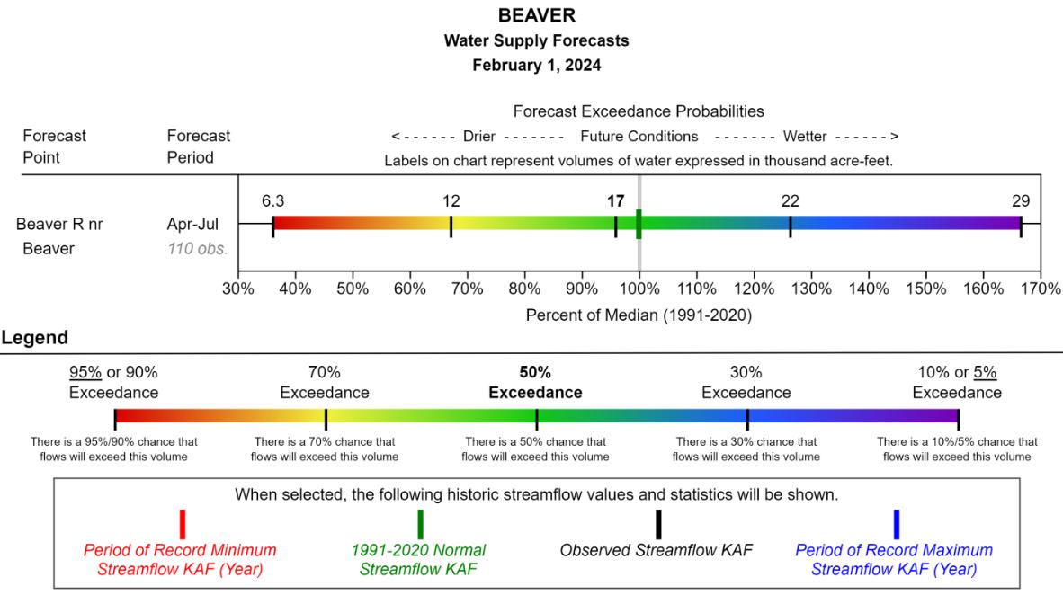
Running out of drinking water or losing crops is not an option. That’s why decision-makers not only need a forecast, they need to know how certain that forecast is. For example, hydrologists often communicate uncertainty using quantile forecasts (see Figure 12.1): A (correct) 90% quantile forecast means that there is a 90% chance that the actual streamflow will be below the forecast and a 10% chance that it will exceed the forecast. Forecasting the 10, 30, 50 (median), 70, and 90 percent quantiles is common.
In fact, in a world with perfect predictions, all quantiles would “collapse” to the same point, but nature does not allow you to peek into her cards so easily. You have to deal with unforeseen weather changes, measurement errors in mountain ranges, and inadequate spatial coverage. This chapter shows you how to integrate these factors into your machine learning pipeline and qualify your predictions with uncertainty estimates.
For a more technical dive into machine learning uncertainty quantification, we recommend [1], [2], [3], and [4], all of which partially inspired our chapter.
All berries are tasty, but some are dangerous. As a result, berry studies has always been one of the best-funded sciences. So asking Rattle to automate berry classification seemed like a natural step. And indeed, after two weeks, Rattle delivered the world’s best berry classifier. The only problem was that nobody trusted the results: The classifier may be right on average, but is it also right for this berry?
12.1 Frequentist vs Bayesian interpretation of uncertainty
Say a hydrologist tells you that there is a 10% probability that the April streamflow in the Beaver River will be less than 6.3 thousand acre-feet. How do you interpret that statement? The possible answers describe one of the oldest discussions within statistics: What is a probability?
Frequentist interpretation
Imagine that you examine the water supply (infinitely) many times under similar conditions, then 10% of the time, you would observe water supplies below 6.3 thousand acre-feet. Frequentists view statements about uncertainty as statements about the relative frequency of events in the long run under similar conditions.
The frequentist interpretation of uncertainty has two central conceptual problems: 1) You simply cannot observe an event with an infinite number of repetitions under similar observational conditions, and it is even unclear whether their relative frequencies are well-defined. 2) You are faced with the so-called reference class problem – what defines relevant similar conditions?
Bayesian interpretation
The hydrologist believes with 10% confidence that the water supply will be less than 6.3 thousand acre-feet. This belief can be expressed in terms of bets she would be willing to make. For example, the hydrologist would be willing to bet up to 10 cents that the water supply will be below 6.3 thousand acre-feet, receiving 1 Dollar if the water supply is actually below 6.3 and nothing if it’s above. To a Bayesian, uncertainty describes subjective degrees of belief. In fact, this subjective belief is constantly updated as new data is observed using the Bayes formula1.
While the Bayesian approach seems to have solved the limitations of the frequentist approach, it faces its own problems: 1) What should you believe if you have not seen any evidence on the matter? This is the so-called problem of prior belief. 2) If uncertainty is a subjective statement about the world, can probabilities be correct? 3) Bayesian probabilities rely on calculating posterior probabilities with the Bayes formula, which is often computationally intractable.
“Probability is the most important concept in modern science, especially as nobody has the slightest notion of what it means.” (Attributed to Bertrand Russell, 1929)
There are also other less established interpretations of uncertainty, such as propensities, likelihoodism, objective Bayesianism, and many others. But whatever understanding of uncertainty you choose, you have to live with its limitations.
Laplace’s Demon: Uncertainties in a deterministic world
Does it matter for the frequentist or Bayesian interpretation of uncertainty whether the world is deterministic or not?
Imagine a hypothetical being with infinite computational resources who knows the location and momentum of every particle in the world. Knowing the laws of nature, could it perfectly determine every past and future state of the world? If so, the world would be deterministic, there would be no uncertainty for that being. This thought experiment of a being with infinite knowledge and infinite computational resources is called the Laplacian Demon. It would be able to precisely calculate the water supply for April.
Does it matter for the interpretation of uncertainty if such a Laplacian Demon exists? Not really! For frequentists, uncertainties are always defined relative to a reference class of similar conditions specified in a particular language. As long as these similar conditions do not determine the event, the uncertainty remains well-defined. Similarly, for Bayesians, uncertainties arise from human computational limitations, incomplete language for the system, insufficient knowledge of the laws, or lack of information about the state of the world. Therefore, both Bayesians and frequentists can reasonably speak of uncertainty at a higher level of description, regardless of whether there is no uncertainty at a lower level for Laplace’s hypothetical demon [5]. This chapter deals with uncertainties that arise from the restriction of the prediction task to certain features, inconclusive reference classes, or simply limited human capacities. We lack the expertise to make sophisticated speculations about potential irreducible uncertainties in the quantum world.
12.3 Uncertainty in predictions, performance & properties
Uncertainty matters whenever you estimate things. Scientists particularly care about the uncertainties in the estimations of predictions, performance, and properties.
Predictions
In the hydrology example, we were concerned with estimating the expected water supply. In this case, we care about the uncertainty in predictions. What is the probability that the water supply will be less than 6.3 thousand acre-feet? What predicted values cover the true label with 95% certainty? What is the variance in predictions from similarly performing models? Prediction uncertainty is the most common concern of researchers using machine learning. Whenever predictions are the basis for action, investigating prediction uncertainties is a key requirement.
Performance
A hydrologist may wish to compare her model with those of a competitor or with the state-of-the-art. This can be done by evaluating the error on historical/future data that was not used to train the model (i.e., the holdout set). However, this provides only a single estimate of the expected error on other unseen data. Therefore, it is often useful to estimate the test error repeatedly and to define confidence intervals. Whenever scientists want to fairly compare the performance of their model with others, they should be transparent about performance uncertainties.
Properties
In a classic statistical modeling context, hydrologists are interested in the uncertainties of model parameters, assuming that they reflect general properties of interest such as (causal) feature effect sizes. In machine learning, parameters such as weights in neural networks often do not lend themselves to such an intuitive interpretation. There are often neither uniquely optimal nor robust parameter settings. To analyze the properties of interest, such as feature effects and importance, you can generalize the notion of parameters to general properties of interest of the data distribution. These properties and their uncertainties can be efficiently estimated, for example, using targeted learning [6]. Alternatively, the same properties and uncertainties can be estimated using post-hoc interpretability techniques [7]. This allows hydrologists to answer questions about the most effective or important feature of water supply.
12.4 Uncertainty quantifies the expected error
When we talk about uncertainty, we are implicitly talking about errors. How close is the predicted water supply to the true future water supply? How close is your test error to the true generalization error? Does the estimated effect of precipitation on water supply match the true effect?
In general terms, you always have a target quantity of interest \(T\) (e.g., true water supply), and your estimate \(\hat{T}\) (e.g., predicted water supply) and you want to know how large the error is, measured by some distance function \(L\): \[ \epsilon:=L(T,\hat{T}) \]
Unfortunately, you don’t have access to \(T\). If you did, you wouldn’t have to estimate anything at all. Therefore, you usually look at the expected error in your estimation, such as the expectation over datasets used in the estimation.
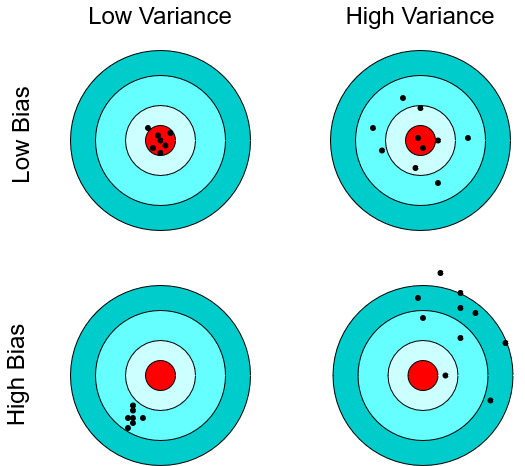
The reason the expected error can be quantified is the so-called bias-variance decomposition, which works for many known distance functions such as the mean squared error or the 0-1 loss [8]:
\[ \underbrace{\mathbb{E}[L(T,\hat{T})]}_{\text{Expected error}} = \underbrace{L(\mathbb{E}[\hat{T}],T)}_{\text{Bias}} + \underbrace{\mathbb{E}[(L(\hat{T},\mathbb{E}[\hat{T}])]}_{\text{Variance}} \]
- Bias describes how the expected estimate differs from the true target value \(T\). In a frequentist interpretation, the idea is that if you repeatedly estimate your target you will be correct on average. A biased estimator systematically underestimates or overestimates the target quantity.
- Variance describes how the estimates vary, for example, for a different data sample. An estimator has high variance if the estimates are highly sensitive to the dataset it receives.
But how does bias-variance decomposition help? For many estimators you can prove unbiasedness, meaning the bias term vanishes. Therefore, the expected error can be fully determined from the variance of the estimate. And the variance can estimated empirically or theoretically.
12.5 Sources of uncertainty
Predictions, performance, and properties are the juicy lemonade you get from our whole machine learning pipeline. Whether the lemonade tastes good depends on the water, the lemons, the squeezing technique, and the ice cubes. A lack of quality in any of these has a direct impact on the quality of your lemonade. Similarly, the expected errors in predictions, performance, and properties are due to errors in our task, modeling setup, and data.
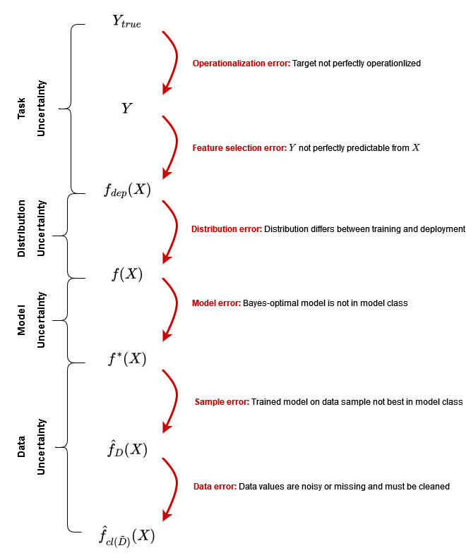
Machine learning modeling can be described as a series of steps. Each of these steps can introduce errors that propagate uncertainty in our estimate. The examples and errors shown in the Figure 12.3 focus on prediction uncertainty, but performance and property uncertainties can be captured in the same way.
12.5.1 Task uncertainty
Specifying a machine learning task means specifying three things: 1. the prediction target \(Y\); 2. a notion of loss \(L\); 3. the input features \(X=(X_1,\dots,X_p)\). In machine learning theory, these three objects are usually considered fixed. In most practical settings, however, they must be chosen carefully.
Prediction target
Often, what you want to predict is vague, making it difficult to operationalize. How do you define the flow of a river? Is one measurement enough? Where to place the sensor? Or should you place multiple sensors and average over many measurements? Vague target variables are especially common in the social sciences. Social scientists are often interested in latent variables that cannot be measured directly. Think of concepts like intelligence, happiness, or motivation. For empirical research, these variables need to be operationalized by some measurable proxy. For example, using grades as a proxy for intelligence, money as a proxy for utility, or hours spent as a proxy for motivation. Operationalizations of latent variables are often debatable, to say the least.
The operationalization error describes the difference between the true prediction target \(Y_{true}\) and its operationalization \(Y\) according to some distance function \(d\): \[ \epsilon_{operationalize}:=d(Y_{true},Y) \]
The operationalization error is a big topic in measurement theory [9], but it still needs to be better bridged to scientific practice [10].
Loss
Uncertainty in the target variable leads to uncertainty in the choice of loss function. The loss function is defined over the co-domain of \(Y\) and if \(Y\) changes, so does the loss \(L\) most of the time. An appropriate loss on the money domain \(]-\infty,\infty[\) differs from the personal happiness evaluation domain \((1,2,\dots,10)\). Even if there is no uncertainty about \(Y\), there can still be uncertainty about the appropriate notion of loss in a given context. Is it better to define prediction error in water supply in terms of absolute distance or should particularly bad predictions be penalized more using the mean squared error?
Input features
You could use many different features to predict a certain target variable, and each combination of features would result in a different prediction. For example, the snow stations could be placed in different locations. But which is the best prediction? It is complicated! When you have multiple models making predictions based on different features, there is not necessarily one prediction model that is always superior. Each of the models may have its merits in different situations. Constraining the prediction task to a subset of input features \(X\) may lead to a feature selection error.
The feature selection error describes the difference between the operationalized target \(Y\) and the Bayes-optimal prediction \(f_{dep}(X)\) according to \(L\) in the deployment distribution (see below in Section 12.5.2 our explanation of Bayes-optimal predictors): \[ \epsilon_{feature}:=L(Y,f_{dep}(X)). \] Adding features with predictive value tends to reduce the error. Thus, one might be interested in the difference between the optimal prediction of \(Y\) based on feature set \(X\) (snow-water equivalent at certain landmarks) and the optimal prediction based on \(X\) plus \(Z\) (weather forecasts). The omitted features error relative to \(X\) describes the difference between the optimal prediction based on \(X\) and the optimal prediction based on \(X\) and \(Z\):
\[ \epsilon_{omitted}:= L(f_{dep}(X,Z),f_{dep}(X)). \]
12.5.2 Interlude: The Bayes-optimal predictor, epistemic, and aleatoric uncertainty
Given a task \((Y,L,X)\), we can define a central concept when it comes to uncertainty – the Bayes-optimal predictor. It describes a prediction function that takes input features \(X\) (e.g., snow-water equivalent, weather forecasts, etc.) and always outputs the best prediction for \(Y\) (i.e., water supply). This does not mean that the Bayes-optimal predictor always predicts the correct amount of water supply. It just gives the best possible guess based on \(X\) only. As we discussed above, the features we have access to, such as snow-water equivalent and weather forecasts, even if perfectly accurate, will usually not completely determine the water supply. Other factors such as the rock layers below the river, the form of the riverbed, or the lakes connected to the river also affect the water supply. The error made by the Bayes-optimal predictor is the feature selection error \(\epsilon_{feature}\) we defined above.
Let’s define the Bayes-optimal predictor more formally. It describes the function \(f: \mathcal{X}\rightarrow \mathcal{Y}\) that minimizes the generalization error (see Chapter 7 or [11]) and is defined pointwise 2 for \(x\in\mathcal{X}\) by:
\[f(x)=\underset{c}{\mathrm{argmin}}\;\;\mathbb{E}_{Y|X}[L(Y,c)\mid X=x].\]
For many loss functions, you can theoretically derive the Bayes-optimal predictor. For example, if you face a regression task and measure loss with the mean-squared error, the optimal predictor is the conditional expectation of \(Y\) given \(X\), i.e. \(f=\mathbb{E}_{Y\mid X}[Y \mid X]\). Alternatively, if you face a classification task and use the \(0-1\) loss, the optimal predictor predicts the class with the highest conditional probability, i.e. \(\mathrm{argmax}_{y\in\mathcal{Y}}\;\;\mathbb{P}(y \mid X)\).
Aleatoric uncertainty, epistemic uncertainty, and why we don’t like the idea of irreducible uncertainties
In the discussion of uncertainty, a common taxonomy is to distinguish between aleatoric and epistemic uncertainty [4]. Aleatoric uncertainty is said to be irreducible. Even with infinite data on snow-water equivalent, weather, and water supply from the past, and fantastic modeling skills, you might still not be able to forecast water supply perfectly – the remaining error is subject to aleatoric uncertainty. Commonly, aleatoric uncertainty is identified with the feature selection error \(\epsilon_{feature}\). Epistemic uncertainty is seen as reducible and stems from your limited access to data, skill in modeling, or computation. For example, if you only have one month of historical data on snow-water equivalent, weather, and water supply, then you have high epistemic uncertainty – collecting more data can reduce this uncertainty.
While we agree that the feature selection error \(\epsilon_{feature}\) is of interest, we disagree with calling it irreducible. As mentioned above, including more features allows you to reduce the error in practice. Uncertainty must always be considered reducible or irreducible only relative to the assumptions that are considered fixed, such as the features, the model, or the data. Whether there is a truly irreducible uncertainty is for physicists to decide, not statisticians.
12.5.3 Distribution uncertainty
The next source of uncertainty is the deployment environment. You simply do not know whether the environment in which you will make your predictions will look exactly like the one you have observed. Over the past 100 years, climate change has significantly altered patterns important to water flow: The best water flow predictions in a given setting in 1940 might look different from the best predictions in 2024. It remains uncertain what environmental conditions will prevail on the Beaver River in the coming years: Will Timpanogos Glacier still be there? How much precipitation can be expected in this area? How many extreme weather events such as droughts or floods will occur?
The distribution error describes the difference in prediction for a given input \(x\) between the Bayes-optimal predictor \(f\) with respect to the training distribution \((X_{train},Y_{train})\) and the Bayes-optimal predictor \(f_{dep}(x)\) with respect to the deployment distribution \((X_{dep},Y_{dep})\):
\[ \epsilon_{distribution}:= L(f_{dep}(x),f(x)) \]
We use \(X\), \(Y\), and \(f\) instead of \(X_{train},Y_{train}, and f_{train}\) to keep the notation easy to read.
12.5.4 Model uncertainty
The Bayes-optimal predictor is a theoretical construct. The best you can do to get it is to approximate it with a machine learning model. To do this, you need to specify what the relationship between \(X\) (e.g. snow-water equivalent) and your target \(Y\) (e.g. water supply) might be. The constraints you place on the model will potentially lead to a model misspecification error.
Model misspecification
Choosing the right model class for a problem is seen as essential, but what is the right class? What kind of relationship should you expect between snow-water equivalent and water supply? How can snow-water equivalent interact with the weather forecast features? This is difficult! Ideally, you want to choose a model class that contains models that are close to or even contain the Bayes-optimal predictor. Since you usually don’t know what the Bayes-optimal predictor looks like, this incentivizes choosing a large model class that allows you to express many possible functions. At the same time, finding the best-fitting model in a large model class is much harder than finding it in a small model class.
Deep neural networks and tree-based ensembles describe highly expressive model classes. They can approximate arbitrary functions well [12], [13], [14] including the Bayes-optimal predictor. Simpler models like linear models or k-nearest neighbors are more constrained in their modeling capabilities.
The bias-variance decomposition provides a good perspective on the uncertainties that can arise from model misspecification. Choosing an expressive model class will reduce the bias in your estimation of the Bayes-optimal predictor. However, it will increase the variance in the estimation process. Conversely, choosing a model class with low expressivity will generally result in a higher bias but lower variance.
Randomness in the hyperparameters selection
One constraint you place on the search for the optimal model within the model class is the hyperparameters. The learning rate in stochastic gradient descent, regularizers like dropout, or the number of allowed splits in random forests, all constrain the models that can effectively be learned. While the search for suitable hyperparameters can in some cases be automated using AutoML methods [15], there remains a random element, as trying out all options always remains computationally intractable.
Random seeds and implementation errors
Most complex learning algorithms contain random elements, for example, bootstrapping in random forests and batch gradient descent in deep learning. This randomness is made reproducible with a seed. Running the same non-deterministic algorithm twice with different seeds will produce different predictions. And, there is generally no theoretical justification for choosing one seed over another. Also, implementation errors in machine learning pipelines can affect the learned model.
Model class, hyperparameters, and seeds constrain the set of effectively learnable models
Together, the choices of model class, hyperparameters, and random seeds constrain the effective model class – i.e. the class of models that can be learned under those choices. We call the learnable model closest to the Bayes-optimal predictor the class-optimal predictor and denote it by \(f^*\).
The model error describes the difference between the Bayes-optimal predictor \(f\) within the training distribution \((X,Y)\) and the class-optimal predictor \(f^*\):
\[ \epsilon_{model}:= L(f(X),f^*(X)). \]
12.5.5 Data uncertainty
Finally, let us look at the ultimate source of uncertainty – the data. You have made measurements in the past and obtained data describing the snow-water equivalent, the weather conditions, and the corresponding water supply. Several things can go wrong:
Sampling
The data you have obtained is only a small sample of the underlying population. With a different sample or more data, your estimate of the label, performance, or property of interest may have looked entirely different.
Uncertainty arising from the data sample can have a large impact on your estimate:
- Randomness: You may have been unlucky and taken a sample that contains many outliers. For example, you took measurements on random days, but they happened to be very rainy days.
- Data size: Your data sample may be too small to be representative of the underlying probability distribution. For example, one measurement per month is not enough for your model to learn the relevant dependencies.
- Selection bias: Your sample may be biased, resulting in a non-representative sample. For example, you may have taken measurements only on dry days to avoid getting wet.
The sample error describes the difference between the prediction of the class-optimal model \(f^*\) and the learned model \(\hat{f}_D\) based on the complete dataset \(D\): \[ \epsilon_{sample}:= L(f^*(X),\hat{f}_D(X)) \]
In the literature, this error is sometimes referred to as the approximation error [4], [16], but we found the term sample error more informative about the nature of this error.
Measurement errors
All data are derived from measurements, or at least it is useful to think of it that way. Your water flow sensors make a measurement. Tracking the amount of snow is a measurement. Even just taking a picture of that snow is a measurement. A measurement error is the deviation of the result of a measurement from the (unknown) true property. It is inevitable to make measurement errors.
- Measurement error in the target introduces a bias. Think of human transcription errors in water flow data.3 There are two directions for this bias: it could be above or below the true property of interest. You might get lucky and biases cancel out on average but that is unlikely, especially if the error is systematic.
- Measurement errors in the features may or may not introduce a bias in the predictions. If there is a random error in the measurement of the snow-water equivalent, it can be washed out during training. Systematic measurement errors in the input features can have more serious consequences: If the snow-water equivalent measurement contains large errors, the model may rely on a proxy feature such as streamflow in the previous month.
Missing data
In an ideal dataset, no cell is empty. Scientific reality is often less tidy. Some values in your rows will look odd: The water flow on March 22 was infinite? The current snow-water equivalent is not a number (NaN)? The date human-entered record is November 32 in 2102? What should we do if some values are missing or undefined?4
There are several reasons why data may be missing:
- Missing completely at random (MCAR): The missing value mechanism is independent of \(X\) and \(Y\). For example, the company that tracks the snow-water equivalent has a server problem and therefore the value is missing.
- Missing at random (MAR): The probability of missingness depends on the observed data. For example, if the guy who sends you the snow-water equivalent sometimes misses it on Thursdays because it is his date night.
- Missing not at random (MNAR): The probability of missingness depends on the missing information. For example, if you don’t get a snow-water equivalent measurement during a snowstorm because the staff can’t reach the sensors.
Measurement errors and missing values lead to another estimation error
Measurement errors and missing values make the data set you deal with in practice look different from the complete data set with unbiased values \(D\) you consider in theory. The data error describes the difference between the learned model \(\hat{f}_D\) based on the complete and accurate dataset \(D\) and the learned model \(\hat{f}_{cl(\tilde{D})}\) on the dataset \(\tilde{D}\) that contains measurement errors and missing values that need to be cleaned up using operations \(cl\):
\[ \epsilon_{data}:= L(\hat{f}_D(X),\hat{f}_{cl(\tilde{D})}(X)). \]
12.6 Quantifying uncertainties
Now we have fancy names for all kinds of sources of uncertainty and the errors they represent. But how can we quantify these uncertainties?
Above we tried to disentangle all kinds of uncertainties: What is the difference between the true target and its operationalization? What is the difference between the Bayes-optimal predictor and the class-optimal model? What is the difference between the class-optimal model and the model learned on an imperfect dataset? In practice, however, you do not have access to the true target, the Bayes-optimal predictor, or the class-optimal model. You always have to run the whole process. The different errors are theoretically well-defined and useful for thinking about minimizing uncertainties, but in practice, the uncertainties are mixed together.
12.6.1 Frequentist vs Bayesian uncertainty quantification
Frequentists and Bayesians approach uncertainty quantification differently.
Frequentists have a simple default recipe – they like repetition. Say you want to quantify the uncertainty in your estimate:
- Assume, or better prove that your estimation is unbiased, i.e. in expectation it will measure the right target quantity.
- Run the estimation process of the target quantity (i.e., predictions, performance, or properties) multiple times under different plausible conditions (e.g., task conceptualization, modeling setup, or data).
- Because of the bias-variance decomposition and the unbiasedness from Step 1, the uncertainty comes exclusively from the variance of the estimates.
This approach has limitations. For example, you cannot prove that your task conceptualization is unbiased. And it can be difficult to come up with multiple plausible conditions for estimation. For frequentist uncertainty quantification, you need confidence in your domain knowledge. But then it is a feasible approach that can be applied post-hoc to all kinds of tasks, models, and data settings. Note, however, that some methods, such as confidence intervals, require additional assumptions that the errors are IID, homoscedastic (i.e., remain the same across different data instances), or Gaussian.
Like frequentists, Bayesians have a standard recipe – they just love their posteriors. Say you want to quantify the uncertainty in your estimate:
- Model the source of uncertainty (e.g. distribution, model, or data) explicitly with a random variable and a prior distribution over that variable.
- Examine how the uncertainty propagates from the source to the target quantity (i.e., predictions, performance, or properties).
- Update the source of uncertainty, and consequently the uncertainty in the target, based on new evidence (e.g., data) using Bayes’ formula.
In terms of uncertainty quantification strategies, we focus mainly on frequentist approaches. Bayesian uncertainty often needs to be baked in from the start, including a refinement of the optimization problem, while frequentist uncertainty is often an easy add-on. But honestly, another reason is that we are just more familiar with frequentist approaches. For a detailed overview of Bayesian uncertainty quantification strategies in machine learning, check out [17] or [18].
12.6.2 Directly optimize for uncertainty
The simplest approach to uncertainty quantification is to predict uncertainties rather than labels. This is often done in classification tasks. Instead of simply predicting the model class with the highest output value, the output values are transformed with a softmax function. The softmax function transforms arbitrary positive and negative values into values that look like probabilities; they are non-negative and sum up to one. When predicting probabilities, you also need different loss functions – the default choices here are cross-entropy and Kullbach-Leibler divergence.
For regression tasks, optimizing directly for uncertainty is less straightforward. Typically, the probability of any individual target value is zero. However, you can estimate the density function directly. This is usually done with Bayesian approaches such as Bayesian regression, Gaussian processes, and variational inference [17]. Here, you explicitly model the uncertainty about the optimal model, either via a Gaussian distribution over functions or parameters, and update the model in light of new data.
More technically, this means that you define a prior distribution \(p(\hat{f})\) over the set of models \(\hat{f}\in F\). Based on this, you can compute the posterior distribution of the models given your data \(p(\hat{f}\mid D)=p(D\mid \hat{f})p(\hat{f})/p(D)\). Finally, this allows us to estimate the target in a Bayesian manner by \[ p(y\mid x, D)=\int_{\hat{f}} p(y\mid \hat{f}) p(\hat{f}\mid x,D)\;d\hat{f}. \] This integral has to be solved numerically again [17].
While you get numbers from direct estimation that look like probabilities, they are often difficult to interpret as such. Especially because they are not calibrated – i.e., they do not match the probabilities in the true outcomes. We discuss how to calibrate probabilities in Section 12.8.
12.6.3 Task uncertainty is hard to quantify
As a reminder, operationalization error describes the difference between the true target (e.g., intelligence) and its operationalization (e.g., IQ test). Quantifying this difference is difficult. There are several challenges: First, the true target is sometimes not directly measurable. Second, even if you had access to the true target and the operationalization, they wouldn’t be on the same scale, making it hard to define a distance function.
What can be done, however, is to look at the coherence or correlations between different operationalizations [2]. For example, in intelligence research, the correlation between different operationalizations of intelligence led to the so-called G-factor, which became the real target that researchers wanted to measure with intelligence tests [19]. Operationalizing the G-factor through multiple specific operationalizations and tests allowed researchers to quantify the operationalization error of specific intelligence tests.
Remember that the feature selection error describes the difference between the operationalized target \(Y\) (like water supply) and the Bayes-optimal predictor given a feature set \(X\) (e.g., snow-water equivalent). It is more tangible to quantify than the operationalization error but it is still difficult. The best proxy for the expected overall feature selection error is the test performance of a well-trained model. For example, if you squeeze the highly engineered water supply prediction model down to a certain test error, the remaining error may arguably be the feature selection error. If you have squeezed out all the predictive value contained in the available features, techniques like cross-validation allow you to additionally estimate the variance in this error.
Quantifying the expected feature selection error for individual instances \(x\) (e.g., the snow-water equivalent and weather forecasts for a given day) is even more difficult. Even if the prediction model as a whole is close to the Bayes-optimal predictor, it may be far off for individual instances \(x\). To see how it might still be possible to quantify the error, check out our discussion of Rashomon sets below.
The omitted feature error can be quantified using interpretability techniques such as leave-one-covariate-out (LOCO) [20] or conditional feature importance [21]. These techniques also allow to quantify uncertainty but always require labeled data of \((X,Z)\).
12.6.4 No distribution uncertainty without deployment data
To estimate distribution uncertainty, we need to know how the training distribution differs from the deployment distribution, or at least have some data from both distributions. If we have access to data, we can compute the respective errors directly. Say one researcher only has access to Beaver River data from 1970 to 1980 while the other has data from July 2014 to July 2024. Both use machine learning algorithms to get the best possible models. Then, they can compare their predictions, performance, or properties on the most recent data to assess the expected distribution error.
Often, we are interested in deployment uncertainty but do not have deployment distribution data. Physical models can the be used to simulate data from different potential distribution shifts. A more detailed discussion on data simulation and augmentation can be found in Chapter 11.
12.6.5 Rashomon sets – many models are better than one
Imagine meeting with ten water supply forecasting experts. Each knows the historical data and has insights into snow-water equivalent and weather forecasts. But they come from different modeling schools, there are physicists, statisticians, machine learners, and so on. Each of them gives you their honest estimate of the water supply in Beaver River for June – but their predictions differ. Not much, but enough to matter. What should you do? There is no good reason to think that any of the ten experts will stand out. The intuitive strategy would be to predict the average (or the median if there are outliers) and analyze the variance in the experts’ opinions to assess the uncertainty in your prediction.
Why not just apply this reasoning to machine learning? Each of the ten experts can be thought of as a different learning algorithm, turning past data into models and current data into predictions. Say you have trained ten models from different model classes, using different hyperparameters and random seeds, all of which perform similarly well. Then this set of models is called a Rashomon set.
Say there is a well-trained model \(\hat{f}_{ref}\) as a reference point and you fix a certain admitted error \(\delta\). Then, \(S:=\lbrace \hat{f}_1,\dots,\hat{f}_k\rbrace\) is a Rashomon set to \(\hat{f}_{ref}\) if for all \(i\in\lbrace 1,\dots,k\rbrace\) holds that the performance of \(\hat{f}_i\) is no worse than \(\delta\), i.e.
\[\mathbb{E}[L(\hat{f}_i(X),Y)] - \mathbb{E}[L(\hat{f}_{ref}(X),Y)] \leq \delta\].
If you assume that your collection of models in the Rashomon set comes from an unbiased estimation process of the optimal model, you can estimate the expected model error by the variance of the predictions in the Rashomon set, i.e.
\[\widehat{\mathbb{V}}_{f^*}[f^*(x)]=\frac{1}{k-1}\sum_{\hat{f}_i\in S}L(\overline{\hat{f}}(x),\hat{f}_i(x)).\]
Assuming a certain distribution of errors (e.g., t-distribution) and IID errors in the Rashomon set, you can use the variance to define confidence intervals. For example, the \(\alpha\) confidence interval for the predictions would be:
\[ CI_{\hat{Y}}=[\hat{f}_{ref}(x)\pm t_{1-\alpha/2}\sqrt{\widehat{\mathbb{V}}_{f^*}[f^*(x)]}] \]
As with all strategies presented here, Rashomon sets can be used to quantify not only the uncertainty in predictions but also the uncertainty in estimated performance and properties. For example, Rashomon sets have been used to quantify the uncertainty in estimating feature importance [22] and feature effects [23]. Similarly, even if the predictions are already probabilities, as is common in classification models, Rashomon sets can be used to quantify higher-order uncertainties. For example, you can obtain imprecise probabilities in the form of intervals by taking the highest and lowest predicted probabilities in the Rashomon set as interval bounds.
Interestingly, in a very Rashomon-set fashion, ensemble methods like random forests implicitly provide an uncertainty quantification of the model error [24]. Each decision tree in the forest can be seen as one prediction model. Similarly, dropout in neural networks can be described as an ensemble method with implicit uncertainty quantification [25].
12.6.6 The key to data uncertainty: sampling, resampling, repeated imputation
The first error we mentioned in the context of data uncertainty is the sample error. In an ideal world, it would be easy to quantify: 1. Take many independent, unbiased samples of different sizes from the same distribution. 2. Quantify the variance in the resulting estimates (i.e., predictions, performance, or properties). This is nice in theory or in simulation studies. But in real life, data is usually both valuable and scarce. You want to use all available data to make your estimates as accurate as possible, not just waste 90% on uncertainty quantification.
Resampling can quantify sample uncertainty, but it can systematically underestimate it
Statisticians have therefore developed smart strategies to avoid wasting data under the umbrella term resampling. The idea: make your best estimate based on the entire dataset. To quantify the sampling uncertainty of that estimate, you study the variance when you repeatedly re-estimate the quantity of interest on different subsets of the full dataset.
There are several approaches to resampling:
- Bootstrapping involves repeatedly drawing samples with replacement.
- In subsampling, you repeatedly draw samples without replacement.
- With cross-validation, you split your data into k-junks of equal size. Cross-validation is particularly useful when you need separate data splits for training and estimation, as in performance estimation (see Chapter 7).
But be careful, with resampling approaches you run the danger of underestimating the variance and consequently the true uncertainty. The reason is that the samples you draw are not really independent. They come from the same overall dataset and share many instances. There are several strategies to deal with the underestimation, such as variance correction strategies like the bias-corrected and accelerated bootstrap [26]. For performance estimation, Nadeau and Bengio [27] suggest several correction factors to tackle underestimation.
Strategies for noisy or missing data
Measurement errors and missing data may look different from the outside, but when you think about it, they are similar. A very noisy feature value can just as well be seen as missing. And, a missing value that is imputed can also be considered noisy. This similarity is reflected in the shared data-cleaning strategies for dealing with them:
- Remove the feature: If a feature is generally super noisy and often missing, we recommend removing it. This way, you can ignore the data error but potentially have a higher feature selection error. Therefore, removing features may be a bad idea if the feature is highly informative about the target. For example, removing the snow-water equivalent from your forecast model will decrease forecast performance.
- Remove individual data points: If the values of a feature are missing completely at random in only a few cases, it may be fine to remove the affected data points. This way, no data uncertainty is introduced. Note that removing data reduces your data size and therefore increases the sampling error. Also, if the missingness or noise is not random, you may introduce selection bias into your dataset.
- Impute missing values: If the missingness is random (MAR), we recommend using data imputation strategies. Ideally, the imputation process takes into account your domain knowledge and data dependencies. Note that imputing missing values based on domain knowledge is itself only a guess. The imputation will sometimes be incorrect.
- Explicitly model uncertainty: If the values of a feature are moderately noisy and you have a guess about how the noise is distributed, we recommend that you model the noise explicitly. This way, the uncertainty can be quantified by propagating the noise forward to the target estimate.
- Improve the measurement: If the missingness is not at random (MNAR), the only good strategy is to get rid of the reason for the missingness and collect new data.
12.7 Minimizing uncertainty
Great, so now you have identified uncertainties and found ways to quantify them – but how do you minimize them? In most contexts, you want to reduce uncertainty: For example, when the water supply model tells you that it is uncertain whether there will be a drought or a flood in the Beaver River. How should you take precautions if the uncertainty is high?
Most, if not all, uncertainties can, in principle, be minimized. Some are just harder to minimize than others. While the goal is to minimize that total uncertainty, the only strategy for doing so is to minimize the individual uncertainties that arise from different sources:
- Task uncertainty
- To minimize the expected operationalization error, put considerable effort into an appropriate operationalization. For example, placing only a single sensor in the river might be a bad idea if the water flows vary along the river.
- To minimize the expected feature selection error, select features that are highly predictive and contain little noise. Omit features that do not add new information to your model.
- Distribution uncertainty
- To minimize the expected distribution error, collect or simulate training data that is representative of the deployment distribution. For example, training your model only on data from the 1970s may be a bad idea given the changed distribution of extreme weather events.
- Model uncertainty
- To minimize model error, choose an appropriate inductive bias in modeling. Strongly constraining the model class and testing a few hyperparameters will result in a high bias. Choosing too broad a model class and unconstrained hyperparameter search will result in high variance. To minimize uncertainty, use your domain knowledge to constrain your model search to a minimal but sufficiently expressive model class to capture the dependency in the data and plausible hyperparameter settings [28]. In water supply forecasting, it is recommended to include physical constraints because they constrain the appropriate model class and consequently reduce model uncertainty [29].
- To find an appropriate model class and hyperparameters, two strategies can be helpful: Either start with simple models and increase complexity until there is no performance gain or start with a complex model and sequentially decrease complexity until there is a performance drop.
- Data uncertainty
- To minimize the expected sample error, the best strategy is to collect more data. Active learning can help you select the data that will reduce uncertainty the most (see the active learning in Chapter 11). However, active learning is impossible in domains like water supply forecasting, where control over the data-generating mechanism is limited.
- Collect multiple labels for an instance to minimize the expected data error in the face of label noise. If there is feature noise, either reduce the noise through improved measurement or replace the feature with an equally predictive but less noisy feature. For example, move a snow sensor from a mountain area with a lot of skiers to a quieter area.
- If the problem is missing data, investigate the cause of the missingness: in many cases, the missingness can be counteracted by a careful measurement, like replacing an unreliable sensor. If the missingness cannot be counteracted, consider removing the feature.
12.8 Calibrating uncertainty measures
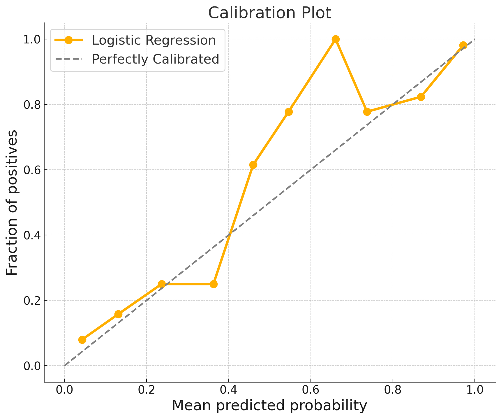
Say you have studied the sources of uncertainty, quantified them, and perhaps even minimized them. Of course, you want to interpret the values in your uncertainty estimates as true probabilities. But there is often a problem with these “probabilities”. The fact that your uncertainty estimate has a 90% confidence does not necessarily mean that the actual probability is 90%. Probabilities can be miscalibrated – the estimated probabilities don’t match the true outcome probabilities.
What does calibration mean in more formal terms? Say you are in a regression setting, such as the water supply forecasting problem. We denote the prediction by \(\hat{Y}\) and the uncertainty estimate for \(\hat{Y}\) with confidence \(c\) by \(u_c(\hat{Y})\). We say that the uncertainties are perfectly calibrated if for all \(c\in[0,1]\) holds:
\[ \mathbb{P}(Y\in u_c(\hat{Y}))=c. \]
For example, the hydrologist’s certainty of 10% that the water supply in the Beaver River will be less than 6.3 thousand acre-feet is calibrated if the actual water supply in the Beaver River is less than 6.3 thousand acre-feet only 10% of the time. Calibration can be similarly defined for classification tasks.
Calibration plots allow you to assess whether probabilities of a classifier are calibrated or not. You compare the predicted and quantified uncertainty with the empirical frequency. For this you pick an outcome class and bin the data points by output score, for example into 0-10%, 10-20%, …, 90-100%. On the x-axes, you plot the confidence bins and on the y-axes the empirical frequencies with which the class matches the chosen class. Figure 12.4 shows an example of a calibration plot, where we compare the mean probabilities with the actual probabilities. If the plot shows a boring linear curve with a slope of 1, congratulations, your model is perfectly calibrated. Evaluating calibration using relative frequencies shows the close relationship between calibration and a frequentist interpretation of probability.
Miscalibration is not just an occasional problem. It is a fair default assumption that any uncertainty estimate is miscalibrated:
- Too short prediction intervals: For the water flow prediction example, we were interested in prediction intervals that cover 80% of the output. The interval was created by predicting the 10% and 90% quantiles. The interval width expresses uncertainty: The larger the interval, the more uncertain the water flow. However, quantile regression has the problem that quantiles are often drawn toward the median [30], an effect that becomes stronger the closer the desired quantile levels are to 0% and 100%. As a result, intervals based on quantile regression tend to be too short and underestimate uncertainty.
- Bootstrapping also undercovers: Remember that in bootstrapping you repeatedly sample data with replacement from the training data. Because the bootstrapped datasets are highly correlated, they underestimate the true uncertainty unless you correct for this bias.
- Bayesian models rely on assumptions: In theory, Bayesian models propagate uncertainty perfectly. You could look at the predictive posterior distribution and, for example, output credible intervals. But they are calibrated (in the frequentist sense) only if your assumptions about likelihood, priors, and so on are correct. Hint: they are unlikely to be correct.
For each miscalibrated uncertainty quantification method, there are several suggestions on how to fix it. For example, to fix miscalibrated probability outputs, you could use post-processing methods such as Platt’s logistic model [31] and Isotonic Calibration. A more general framework for dealing with all these problems is conformal prediction, which can make any uncertainty measure “conformal” – with coverage guarantees.
Conformal prediction, a set-based approach to uncertainty
Standard uncertainty quantification treats models and predictions as fixed and returns the uncertainties. Conformal prediction takes the opposite approach: The modeler must specify the desired confidence level (related to uncertainty), and a conformal prediction procedure changes the model output to conform to the confidence level. Consider water supply forecasting: Normally, you would simply predict a scalar value and provide the quantified uncertainty estimate in some form. With conformal prediction, you first set a confidence level and then modify your confidence interval to cover the true value with the desired confidence. Thus, conformal prediction comes with a coverage guarantee – at least for data that is exchangeable, the prediction set corresponds to the desired confidence level. But beware, the coverage guarantee is often marginal, i.e. it only applies to the average of the data.
Conformal prediction is more than a simple algorithm, it is a whole framework that allows to conformalize different uncertainty scores:
- Turn a quantile interval into a conformalized quantile interval [32]).
- Turn a class probability vector into a set of classes [33].
- Turn a probability score into a probability range (Venn-ABERS predictor) [34].
There is a simple recipe for conformal prediction – training, calibration, and prediction.
- Training:
- You split the training data into training and calibration data.
- Train the model using the training data.
- Calibration:
- Compute uncertainty scores (also called nonconformity scores) for the calibration data.
- Sort the scores from certain to uncertain (low to high).
- Decide on a confidence level.
- Find the quantile where \(1-\alpha\) of the nonconformity scores are smaller.
- Prediction:
- Compute nonconformity scores for the new data.
- Select all predictions that produce a score below \(\hat{q}\).
- These predictions form the prediction set/interval.
Nothing comes for free and neither does conformal prediction. The “payment” is the additional calibration data you need, which can complicate the training process. Small calibration sets will lead to large prediction sets, possibly to the point where they are no longer useful. Furthermore, the calibration data must be interchangeable with the training data, which can be a problem with time series data, for example. However, there are also conformal procedures for time series that rely on a few more assumptions. Otherwise, conformal prediction is a very versatile approach.
To learn more about conformal prediction, check out the book Introduction to Conformal Prediction with Python.
12.9 Understand uncertainty to gain knowledge
In this chapter, you learned about the many different sources of error in machine learning pipelines and how they introduce uncertainty into your estimates. While uncertainty can be disentangled in theory, it is difficult to disentangle in practice – you can usually only quantify the overall uncertainty. Nevertheless, it is helpful to separate uncertainties conceptually, especially if you are looking for strategies to minimize uncertainty.
Uncertainty should not be seen as just an add-on. Uncertainty quantification is essential, especially if you want to gain new knowledge with machine learning or act on machine learning predictions. To get a realistic picture of the true uncertainty, all sources of uncertainty should be considered
When it comes to quantifying uncertainty, we recommend that scientists be pragmatists. You can use Bayesian techniques if you have domain knowledge that allows you to set a reasonable prior. Otherwise, frequentist approaches to uncertainty quantification can provide you with (calibrated) uncertainties under modest assumptions.
Uncertainty is closely related to many chapters in this book:
- Theoretically, the roots of uncertainty quantification lie in our theory of generalization from Chapter 7. Concepts such as generalization error, cross-validation, or biased sampling can be found in both chapters.
- Many approaches to minimizing uncertainty rely on domain knowledge (see Chapter 8). Reliable domain knowledge can significantly minimize task, distribution, model, and data uncertainty.
- The uncertainty framework presented here is quite general. It can be applied to interpretability techniques (see Chapter 9) and even to causal effect estimation (see Chapter 10).
- Uncertainty has close ties to the robustness in Chapter 11, especially when it comes to distribution uncertainty and strategies to reduce data uncertainty like active learning. Conceptually, the link is that robustness gives guarantees for worst-case error, while uncertainty gives guarantees in expectation [35].
We hope we have minimized your uncertainty about uncertainty with this chapter…
Bayes formula describes how to update your prior beliefs in light of new evidence. Namely, if \(\hat{f}\) is your hypothesis and \(D\) is your evidence, you should update your belief with: \(\mathbb{P}(\hat{f}\mid D)=\frac{\mathbb{P}(D\mid \hat{f})\mathbb{P}(\hat{f})}{\mathbb{P}(D)}.\)↩︎
Technical detail: For \(X=x\) with a probability of zero, the term on the right is undefined. Therefore, the Bayes-optimal predictor does not describe a unique function, but an equivalence class of functions that are aligned at \(x\) with positive density.↩︎
Many of these measurements from gauges and snow stations are fully automated. But for the sake of illustration, let’s assume they are recorded by humans.↩︎
We do not talk about whole entries missing here, because this typically leads to problems of representativeness and is covered in Chapter 7.↩︎